Conceptual Foundation & Intuitive Analogy
🧭 Conceptual Foundation & Pattern Intuition
Graph traversal models arbitrary systems of interconnected entities. A graph consists of vertices (states, grid cells, entities) and edges (dependencies, roads, cardinal adjacencies). Unlike trees, general graphs may contain cycles and disconnected components. Graph algorithms systematically explore reachable states using either Depth-First Search (DFS, diving deeply down one branch using a LIFO stack) or Breadth-First Search (BFS, expanding concentrically outward level by level using a FIFO queue). The cardinal rule of graph traversal is the visited set invariant: every discovered node must be recorded immediately upon discovery to prevent infinite loops on cyclic edges and redundant work across dense connections.
The abstract template above generalizes this to any "count the connected clusters" question: get_neighbours and is_interesting are the only holes a concrete problem needs to fill in. The next archetype, Number of Islands, fills those holes concretely and walks through the exact flood-fill analogy and code this shape produces.
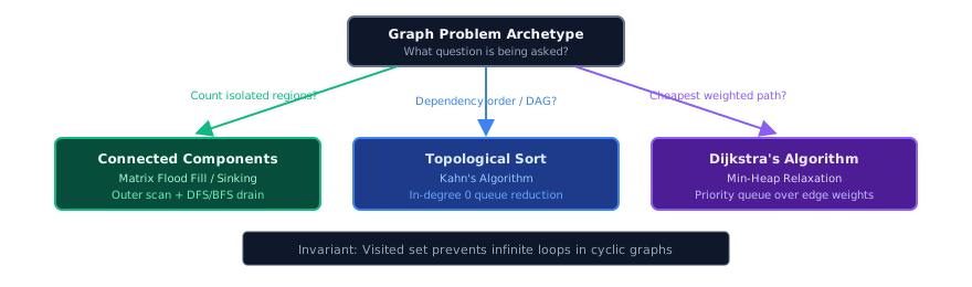
Every node is processed exactly once. The visited marker is what turns a possibly-infinite walk into O(V + E).
Maintains visited set or 3-color states (WHITE=unvisited, GREY=visiting/cycle, BLACK=processed) across adjacency lists.
Loop outer vertices 0..V-1 to handle disconnected subgraphs; explore edges via BFS/DFS/PriorityQueue.
The 6 Mental Models of Graph Algorithms
Classify graph problems by connectivity, directionality, and edge weights.
1Flood Fill
2D grid / graph ➔ outer unvisited discovery ➔ consume full componentConnected Components (Number of Islands / Flood Fill)
| 1 | from typing import Callable, Dict, Hashable, Iterable, List |
| 2 | |
| 3 | |
| 4 | def flood_fill(cells: Iterable[Hashable], is_land: Callable[[Hashable], bool], neighbors: Callable[[Hashable], Iterable[Hashable]]) -> Dict[Hashable, int]: |
| 5 | """Flood Fill: label every land cell with the number of its group of connected land |
| 6 | cells. |
| 7 | Precondition: neighbors is symmetric. If b is a neighbour of a, then a is a |
| 8 | neighbour of b. |
| 9 | Groups are numbered 0, 1, 2, ... in scan order, so the number of groups is |
| 10 | max(group.values()) + 1. |
| 11 | V = cells. T = the cost of one is_land or neighbors call (neighbors yields at most T |
| 12 | cells). |
| 13 | Time: O(V * T) | Space: O(V) |
| 14 | """ |
| 15 | # Maps every already-searched land cell to its group number |
| 16 | group: Dict[Hashable, int] = {} |
| 17 | count = 0 |
| 18 | |
| 19 | for cell in cells: |
| 20 | # 1. Find An Unlabeled Land Cell: |
| 21 | # A cell with no group yet and is_land(cell) true has not been reached by any |
| 22 | # earlier search, so it starts a brand-new group. |
| 23 | if is_land(cell) and cell not in group: |
| 24 | # A new group: count grows once per search, not per cell |
| 25 | group[cell] = count |
| 26 | stack = [cell] |
| 27 | |
| 28 | # 2. Flood The Whole Group: |
| 29 | # The loop keeps running until stack is empty, so every cell reachable from |
| 30 | # this one is labeled before the outer loop is allowed to move on. |
| 31 | while stack: # Inner search uses up the whole group |
| 32 | curr = stack.pop() |
| 33 | for nxt in neighbors(curr): |
| 34 | if is_land(nxt) and nxt not in group: |
| 35 | group[nxt] = count # Label on push, not on pop |
| 36 | stack.append(nxt) |
| 37 | |
| 38 | # 3. Advance The Group Counter: |
| 39 | # count only changes once the whole group has been labeled, so the next |
| 40 | # brand-new cell starts the next number. |
| 41 | count += 1 |
| 42 | |
| 43 | return group |
Scan every cell, and when you meet a "1" that no search has reached, add one to islands and flood that cell's whole island with the inner stack search. The inner search turns every connected land cell to "0", so the outer scan never meets that island again and counts it exactly once. The trap is where the counter lives: islands += 1 belongs in the outer scan, once per search, never inside the inner loop, where it would count cells instead of islands.
Gotcha 1 of 4
- The trap
Gotcha 1: Adding to
islandsinside the inner search loopMistakeif 0 <= nr < R and 0 <= nc < C and grid[nr][nc] == "1": grid[nr][nc] = "0" islands += 1 stack.append((nr, nc))Fixif 0 <= nr < R and 0 <= nc < C and grid[nr][nc] == "1": grid[nr][nc] = "0" stack.append((nr, nc))What happens: The outer scan adds 1 to
islandsfor the first cell of an island. The inner loop then adds 1 again for every other cell it reaches. Soislandsends as the number of land cells, not the number of islands.islands += 1belongs in the outer scan, once per new search.Example: Number of Islands (LC 200): grid = [["1", "1"], ["0", "1"]]Mistake: returns 3Fix: returns 1
2Kruskal's MST
edge list sorted by weight ➔ union by rank/size ➔ connect componentsMinimum Spanning Tree (Kruskal's, built on Union-Find)
| 1 | from typing import List |
| 2 | |
| 3 | def kruskal_mst(n: int, edges: List[List[int]]) -> int: |
| 4 | """Kruskal's MST (Connecting Cities With Minimum Cost): cheapest total cost to join |
| 5 | nodes 1..n, or -1. |
| 6 | Time: O(E log E) | Space: O(V) |
| 7 | """ |
| 8 | parent = list(range(n + 1)) |
| 9 | |
| 10 | def find(x: int) -> int: |
| 11 | while parent[x] != x: |
| 12 | parent[x] = parent[parent[x]] # Path halving: skip a level on every step |
| 13 | x = parent[x] |
| 14 | return x |
| 15 | |
| 16 | edges.sort(key=lambda e: e[2]) # Cheapest edges first |
| 17 | mst_cost = 0 |
| 18 | edges_count = 0 |
| 19 | |
| 20 | for u, v, w in edges: |
| 21 | root_u, root_v = find(u), find(v) |
| 22 | if root_u != root_v: # Different groups: this edge is safe to take |
| 23 | parent[root_u] = root_v # Join the roots, not the nodes |
| 24 | mst_cost += w |
| 25 | edges_count += 1 |
| 26 | if edges_count == n - 1: |
| 27 | break # A spanning tree has exactly n - 1 edges |
| 28 | |
| 29 | return mst_cost if edges_count == n - 1 else -1 # Fewer edges: not connected |
Sort edges by weight and take each edge whose ends have different roots, find(u) != find(v), joining the two groups. The cheapest edge between two separate groups is always safe to take: any full wiring must cross that gap somewhere, and swapping in the cheaper edge never costs more; an edge whose ends already share a root would only close a cycle, so skipping it loses nothing. The trap is the final check: fewer than n - 1 edges taken means the graph is not connected, so return -1 instead of the partial cost.
Gotcha 1 of 4
- The trap
Gotcha 1: Returning
mst_costwithout checkingedges_countMistakereturn mst_costFixreturn mst_cost if edges_count == n - 1 else -1What happens: A tree that joins
nnodes has exactlyn - 1edges. If the edges run out with fewer, some cities are still in separate groups.mst_costis then the cost of a partial wiring. The problem asks for-1in that case.Example: Connecting Cities With Minimum Cost (LC 1135): n = 4, connections = [[1, 2, 3], [3, 4, 4]]Mistake: returns 7Fix: returns -1
3Dijkstra
weighted directed graph ➔ min-heap (dist, node) ➔ greedy relaxationDijkstra's Algorithm
| 1 | import heapq |
| 2 | from typing import List, Dict |
| 3 | |
| 4 | def dijkstra(n: int, edges: List[List[int]], source: int) -> Dict[int, float]: |
| 5 | """Dijkstra (the core of Network Delay Time): cheapest distance from source to nodes |
| 6 | 1..n. |
| 7 | Time: O((V + E) log V) | Space: O(V + E) |
| 8 | """ |
| 9 | adj = [[] for _ in range(n + 1)] |
| 10 | for u, v, w in edges: |
| 11 | adj[u].append((v, w)) |
| 12 | |
| 13 | dist = {i: float('inf') for i in range(1, n + 1)} |
| 14 | dist[source] = 0 |
| 15 | pq = [(0, source)] # (cost, node) |
| 16 | |
| 17 | while pq: |
| 18 | d, u = heapq.heappop(pq) |
| 19 | if d > dist[u]: |
| 20 | continue # Stale entry: u was already settled with a smaller d |
| 21 | |
| 22 | for v, weight in adj[u]: |
| 23 | if dist[u] + weight < dist[v]: # Relax the edge |
| 24 | dist[v] = dist[u] + weight |
| 25 | heapq.heappush(pq, (dist[v], v)) |
| 26 | |
| 27 | return dist |
Keep a min-heap pq of (distance, node) pairs. Popping the smallest d settles u, because with non-negative weights any other path to u leaves the settled area through a node that is at least as far away, so it can't be shorter. For each edge, if going through u is shorter, update dist[v] and push the new pair. The trap is the stale entry: u can sit in pq several times, so skip it when d > dist[u]; without that line the answer stays right, but old entries relax every edge again and the run can slow down badly.
Gotcha 1 of 4
- The trap
Gotcha 1: Relaxing edges from a stale heap entry
Mistaked, u = heapq.heappop(pq)Fixd, u = heapq.heappop(pq) if d > dist[u]: continueWhat happens:
uis pushed again every timedist[u]improves. Sopqcan hold old pairs foruwith a largerd. Without the check, an old pair relaxes every edge ofuagain. The answer stays right, because an olddnever improvesdist[v]. But the run can do much more work. That is why this mistake has no example.
4Eulerian Path
edges ➔ walk and delete each used edge ➔ nodes appended when stuck, then reversedEulerian Path (Hierholzer's Algorithm)
| 1 | from collections import defaultdict |
| 2 | from typing import Hashable, List |
| 3 | |
| 4 | def eulerian_path(edges: List[List[Hashable]]) -> List[Hashable]: |
| 5 | """Eulerian Path (Hierholzer's algorithm, the core of Reconstruct Itinerary): the |
| 6 | smallest walk that uses every directed edge exactly once. |
| 7 | Time: O(E log E) | Space: O(E) |
| 8 | """ |
| 9 | graph = defaultdict(list) |
| 10 | balance = defaultdict(int) # out-degree minus in-degree |
| 11 | # reverse order, so pop() takes the smallest neighbour |
| 12 | for u, v in sorted(edges, reverse=True): |
| 13 | graph[u].append(v) |
| 14 | balance[u] += 1 |
| 15 | balance[v] -= 1 |
| 16 | # one extra edge out starts the path; a circuit starts at the smallest node |
| 17 | start = next((x for x in graph if balance[x] == 1), min(graph)) |
| 18 | path, stack = [], [start] |
| 19 | while stack: |
| 20 | node = stack[-1] |
| 21 | if graph[node]: |
| 22 | stack.append(graph[node].pop()) # follow an unused edge and delete it |
| 23 | else: |
| 24 | # no edge left: node is final in the rest of the walk |
| 25 | path.append(stack.pop()) |
| 26 | return path[::-1] # nodes were finished last-first |
Walk from start, deleting each edge as you follow it with stack.append(graph[node].pop()), and add a node to path only when it has no unused edge left, with path.append(stack.pop()); reversing path gives the walk. This is correct because a walk that always takes some unused edge can only get stuck at the node where the whole path must end, so the first node to run out of edges is the last node of the answer; any cycle the walk skipped hangs off a node that is still on stack, and it is walked, and placed, when the stack backs up to that node. The trap is writing a node into the answer when you first reach it: the walk can enter the final dead end before a cycle has been used (in Reconstruct Itinerary (LC 332), taking the smallest airport first can strand the tickets of a loop), so a node goes into path only once its edges are used up, and the list is reversed at the end.
Gotcha 1 of 4
- The trap
Gotcha 1: Writing each node into the answer when first reached
Mistakepath.append(node) while graph[node]: node = graph[node].pop() path.append(node)Fixif graph[node]: stack.append(graph[node].pop()) else: path.append(stack.pop())What happens: The walk can enter the final dead end before a cycle has been used. Written in the order reached, the answer stops at that dead end. The cycle's edges are never used. The blueprint adds a node to
pathonly when its edges are used up, then reversespath.Example: Reconstruct Itinerary (LC 332): tickets = [["JFK", "KUL"], ["JFK", "NRT"], ["NRT", "JFK"]]Mistake: returns ['JFK', 'KUL']Fix: returns ['JFK', 'NRT', 'JFK', 'KUL']
5Floyd-Warshall
distance table ➔ allow one more middle node per round ➔ all shortest distancesFloyd-Warshall (All-Pairs Shortest Path)
| 1 | from typing import List |
| 2 | |
| 3 | def floyd_warshall(n: int, edges: List[List[int]]) -> List[List[float]]: |
| 4 | """Floyd-Warshall (the core of Course Schedule IV): shortest distance between every |
| 5 | pair of nodes. |
| 6 | Time: O(V^3) | Space: O(V^2) |
| 7 | """ |
| 8 | dist = [[float("inf")] * n for _ in range(n)] |
| 9 | for i in range(n): |
| 10 | dist[i][i] = 0 # a node reaches itself at distance 0 |
| 11 | for u, v, w in edges: |
| 12 | # directed edge u -> v; keep the lighter of two parallel edges |
| 13 | dist[u][v] = min(dist[u][v], w) |
| 14 | for k in range(n): # k OUTERMOST: allow node k as a stop |
| 15 | for i in range(n): |
| 16 | for j in range(n): |
| 17 | if dist[i][k] + dist[k][j] < dist[i][j]: |
| 18 | dist[i][j] = dist[i][k] + dist[k][j] # go through k |
| 19 | return dist |
Allow the nodes as stops one at a time: for each k, let every pair i, j go through k when dist[i][k] + dist[k][j] < dist[i][j]. This is correct because, once k is allowed, the shortest i -> j path with stops in 0..k either avoids k, and is already in dist[i][j], or passes through k once and splits into an i -> k part and a k -> j part whose stops lie in 0..k - 1, and both of those are already in the table. The trap is the loop order: for k in range(n) must be the outermost loop. With k inside the i and j loops, dist[i][k] is read before the paths through the smaller stops have been allowed, and some pairs keep a distance that is too long, or no path at all.
Gotcha 1 of 4
- The trap
Gotcha 1: Putting
for k in range(n)inside theiandjloopsMistakefor i in range(n): for j in range(n): for k in range(n):Fixfor k in range(n): for i in range(n): for j in range(n):What happens: With
kinnermost, the pair(i, j)is finished before the other pairs are updated.dist[i][k]may still miss a path through a smaller stop. So some pairs keep a distance that is too long, or no path at all.Example: n = 4, edges = [[0, 3, 1], [3, 2, 1], [2, 1, 1]], read dist[0][1]Mistake: returns infFix: returns 3
6Tarjan's Bridges
DFS tree ➔ discovery time and low-link per node ➔ bridge when low[child] > disc[parent]Tarjan's Bridges & Articulation Points
| 1 | from typing import List |
| 2 | |
| 3 | def find_bridges(n: int, edges: List[List[int]]) -> List[List[int]]: |
| 4 | """Tarjan's Bridges (the core of Critical Connections in a Network): every edge |
| 5 | whose removal disconnects the graph. |
| 6 | Time: O(V + E) | Space: O(V + E) |
| 7 | """ |
| 8 | graph = [[] for _ in range(n)] |
| 9 | for i, (u, v) in enumerate(edges): |
| 10 | graph[u].append((v, i)) |
| 11 | graph[v].append((u, i)) |
| 12 | # discovery time; -1 = not reached yet |
| 13 | disc = [-1] * n |
| 14 | # earliest disc the subtree reaches with one back edge |
| 15 | low = [0] * n |
| 16 | bridges = [] |
| 17 | time = 0 |
| 18 | for root in range(n): |
| 19 | if disc[root] != -1: |
| 20 | continue |
| 21 | disc[root] = low[root] = time |
| 22 | time += 1 |
| 23 | # (node, edge id we came in by, next neighbour index) |
| 24 | stack = [(root, -1, 0)] |
| 25 | while stack: |
| 26 | node, in_edge, idx = stack[-1] |
| 27 | if idx < len(graph[node]): |
| 28 | stack[-1] = (node, in_edge, idx + 1) |
| 29 | nxt, edge = graph[node][idx] |
| 30 | if edge == in_edge: |
| 31 | continue # not the tree edge back to the parent |
| 32 | if disc[nxt] == -1: |
| 33 | disc[nxt] = low[nxt] = time # tree edge: go deeper |
| 34 | time += 1 |
| 35 | stack.append((nxt, edge, 0)) |
| 36 | else: |
| 37 | # back edge: reaches an earlier node |
| 38 | low[node] = min(low[node], disc[nxt]) |
| 39 | else: |
| 40 | stack.pop() # node is finished |
| 41 | if stack: |
| 42 | parent = stack[-1][0] |
| 43 | low[parent] = min(low[parent], low[node]) |
| 44 | # nothing below node climbs to parent or above |
| 45 | if low[node] > disc[parent]: |
| 46 | bridges.append([parent, node]) |
| 47 | return bridges |
Number the nodes in DFS order with disc, and let low[node] be the earliest disc that node's subtree can reach through one edge other than the tree edge it came in by; when node finishes, the tree edge parent -> node is a bridge exactly when low[node] > disc[parent]. This is correct because any other route between the two sides of that edge has to leave node's subtree by some edge, and an undirected DFS has no edges across subtrees, so that edge climbs to parent or above and would make low[node] <= disc[parent]. The trap is the comparison: bridges need the strict low[node] > disc[parent]. With >=, which is the test for articulation points, an edge whose subtree climbs back exactly to parent (so it sits on a cycle) is wrongly reported.
Gotcha 1 of 4
- The trap
Gotcha 1: Testing
low[node] >= disc[parent]instead of>Mistakeif low[node] >= disc[parent]:Fixif low[node] > disc[parent]:What happens:
low[node] == disc[parent]means the subtree ofnodeclimbs back exactly toparent. So the edgeparent -> nodelies on a cycle, and removing it disconnects nothing.>=reports it anyway.>=is the test for articulation points, not for bridges.Example: Critical Connections in a Network (LC 1192): n = 4, connections = [[0, 1], [1, 2], [2, 0], [1, 3]]Mistake: returns [[1, 3], [0, 1]]Fix: returns [[1, 3]]
Built on the mental models above
- Cycle DetectionCycle Detection in a Directed Graph (DFS Three-Color)
A node has three states, not seen, on the current path and finished, and reaching a node on the current path proves a cycle.
- Strongly Connected ComponentsStrongly Connected Components (Kosaraju / Tarjan)
Record the finish order, then search the reversed graph in reverse finish order, and each search finds one group.
- Bipartite CheckBipartite Graph (Two-Coloring)
Each node gets one of two sides, a neighbour gets the other side, and an edge inside one side means the answer is no.
- Undirected CycleCycle Detection in an Undirected Graph (Parent Check)
The search remembers the node it came from, and reaching an already-seen node that is not that parent proves a cycle.
- Graph PathsTraverse an Adjacency List and Carry a Result (All Paths From Source to Target)
The graph is an adjacency list, and the walk carries a path that it extends, copies at the target and restores. No visited set: every path counts.
- Bellman-FordBellman-Ford (K-Stop Relaxation)
Edges are relaxed in rounds instead of popping the cheapest node, so a path is limited to a number of edges and negative weights are allowed.
- A Star SearchA* Search (Cost So Far Plus a Guess)
The heap orders states by the cost so far plus a guess of the cost still to go, and the guess must never be too large.
- Tarjan SCCTarjan's Strongly Connected Components (One Pass with Low-Link)
The same discovery time and low-link run on a directed graph with a stack, and a node whose low-link equals its own discovery time is the root of one group.
The Graphs Decision Rule
When facing an unseen graph problem, ask in this order:
Scan every cell or node; each unvisited one starts a new group, and a DFS or BFS marks its whole group visited.
Color each component by BFS or DFS, alternating colors; an edge between two nodes of the same color means it is not bipartite.
Build graph and run Kahn's algorithm (in_degree == 0 queue).
Color nodes WHITE, GREY while on the DFS path and BLACK when finished; reaching a GREY node means a cycle.
Use min-heap with distance relaxation and stale-entry guard.
Order the heap by cost + guess(state), skip a stale entry, and check the goal when it is popped, not when it is pushed.
Relax every edge k + 1 times, each round reading only the previous round's distances.
dist[i][j] = min(dist[i][j], dist[i][k] + dist[k][j]), with k as the outer loop.
Sort edges by weight and keep each edge whose ends Union-Find reports as not yet connected.
DFS with discovery times and low-links; edge (u, v) is a bridge when low[v] > disc[u].
Record DFS finish order, reverse every edge, then DFS in reverse finish order; each tree is one group.
Run one DFS with discovery times, low-links and a stack of waiting nodes; pop a group whenever a node's low-link equals its discovery time.
Walk unused edges until stuck, add the stuck node to the route on the way back, then reverse the route.
Search from a node and remember the node it came from; an edge to a seen node that is not that parent closes a cycle, and a tree also needs every node reached.
Walk the adjacency list with one shared path: append before the call, pop after it, save a copy at the target, and keep no visited set.
Pattern Architecture & Invariant Design Masterclass
A graph is the most general shape data comes in: a set of nodes, and a set of connections between them. That is all. There is no root, there is no "first" node, and — the part that changes everything — a path can lead you back to where you started.
Trees are graphs with the loops removed and a root chosen. Every technique in dfs.md and bfs.md still applies, plus one mandatory addition:
You must remember where you have already been. Without a
visitedset, a single cycle makes the traversal run forever.
Three sub-problems cover almost every graph question in an interview, and telling them apart is the actual skill:
- "How many separate pieces are there?" → Traverse from every unvisited node; each traversal you start is one new piece.
- "In what order can I do these tasks, given that some must come before others?" → Topological sort. Only possible when the graph has no cycles.
- "What is the cheapest route, when steps cost different amounts?" → Dijkstra. BFS is wrong here, and knowing why is the point.
🔬 Variable Anatomy: The 7 Variables Every Graph Algorithm Uses
To connect abstract graph concepts with concrete Python syntax, here is the universal code anatomy showing what every variable does:
from collections import defaultdict, dequeimport heapq def graphMasterTemplate( num_nodes: int, edges: list[list[int]], source: int) -> dict[int, int]: # ========================================================================= # 1. THE TOPOLOGY & STATE STORAGE POOLS # ========================================================================= adj = defaultdict(list) # 🕸️ Graph Adjacency List: node -> list of (neighbor, weight) in_degree = [0] * num_nodes # 📥 Prerequisite Counter: tracks incoming DAG(Directed Acyclic Graph) edges visited = set() # 🚫 Visited Deduplication Set: prevents infinite cycles dist = {source: 0} # ⏱️ Shortest Distance Table: tracks minimal cost to each node # ========================================================================= # 2. THE GRAPH BUILD PHASE # ========================================================================= for u, v, w in edges: adj[u].append((v, w)) in_degree[v] += 1 # In-degree populated for topological sorting # ========================================================================= # 3. FRONTIER PROCESSING PIPELINE (DIJKSTRA / BFS / KAHN'S) # ========================================================================= # Min-heap priority queue storing (current_distance, node_id) min_heap = [(0, source)] while min_heap: d, u = heapq.heappop(min_heap) # ⚠️ CRITICAL: Stale-entry guard for lazy Dijkstra heap relaxation if d > dist.get(u, float('inf')): continue visited.add(u) for v, weight in adj[u]: new_dist = d + weight if new_dist < dist.get(v, float('inf')): dist[v] = new_dist heapq.heappush(min_heap, (new_dist, v)) # ⚡ Edge relaxation return dist Variable Role Reference:
| Variable | Role in Code | Question It Answers | ❌ What Happens If Omitted or Mismanaged? |
|---|---|---|---|
adj | defaultdict(list) | "Who are my direct outgoing neighbors and edge weights?" | ❌ Without an adjacency map, querying neighbors requires scanning the entire edge list on every step (). |
visited | Hash set / boolean table | "Have I already scheduled or processed this vertex?" | ❌ Without visited, traversing a cyclic graph enters an infinite loop and crashes with call-stack/memory overflow. |
in_degree | Integer array / map | "How many unmet prerequisites block this task from executing?" | ❌ In Topological Sort (Kahn's), without tracking in-degree, dependent tasks execute prematurely out of topological order. |
queue / stack | deque or list | "Which node is next in line for BFS level-order or DFS depth traversal?" | ❌ Using list.pop(0) turns BFS into an unacceptable bottleneck. |
dist | Distance lookup table | "What is the absolute cheapest cost known to reach vertex ?" | ❌ Without maintaining a distance table, Dijkstra's algorithm cannot determine if an edge represents a valid relaxation. |
min_heap | Priority queue [(d, u)] | "Which unfinalized node currently has the globally smallest provisional distance?" | ❌ Using a standard FIFO queue on weighted graphs produces incorrect non-shortest paths. |
components | Integer accumulator | "How many isolated, disconnected clusters exist across the graph?" | ❌ Incrementing components inside the inner flood-fill traversal counts individual vertices instead of disjoint components. |
🧠 The Universal Representation Contract:
In graph algorithms, graph structure is represented in two standard ways:
- Explicit Adjacency List (
adj[u] = [v1, v2]): Used for sparse node-and-edge graphs (e.g. Course Schedule, Network Delay). Built once in before traversal.- Implicit Coordinate Grids (
dr, dc = [(-1,0), (1,0), (0,-1), (0,1)]): Used for 2D matrices (e.g. Number of Islands, Walls and Gates). Neighbors are dynamically computed on-the-fly without allocating adjacency lists.
🌟 The 3 Dimensions of Graph Algorithms & The Cycle-Breaker Principle
Every graph problem is governed by 3 Fundamental Dimensions:
┌─────────────────────────────────────────────────────────────────────────────┐│ THE 3 DIMENSIONS OF GRAPH ALGORITHMS │├───────────────────┬───────────────────────────────────┬─────────────────────┤│ Dimension │ Mechanism in Code │ Question It Answers │├───────────────────┼───────────────────────────────────┼─────────────────────┤│ 1. FRONTIER ORDER │ Queue (BFS), Stack (DFS), │ "Which node gets ││ (Discipline) │ or Min-Heap (Dijkstra) │ processed next?" │├───────────────────┼───────────────────────────────────┼─────────────────────┤│ 2. EDGE DYNAMICS │ Unweighted (step count), │ "How is transition ││ (Weights/Dir) │ Directed DAG(Directed Acyclic Graph), or Weighted edges │ cost evaluated?" │├───────────────────┼───────────────────────────────────┼─────────────────────┤│ 3. CYCLE CONTROL │ `visited` set, in-degree counter, │ "How do we prevent ││ (Loop Breaker) │ or 3-color state machine │ infinite loops?" │└───────────────────┴───────────────────────────────────┴─────────────────────┘ How this plays out in actual problems:
🟢 Scenario A: Connected Components & Grid Flood Fill (Using Outer Scan + Sink)
- In connected component problems (like Number of Islands), we want to count separate isolated clusters.
- The Rule: The outer loop scans every cell. When it hits an unvisited land cell, increment
components += 1and launch a traversal to sink the entire island so the outer loop never sees it again. - The Code:
if grid[r][c] == '1': count += 1; dfs(r, c)
🔵 Scenario B: Topological Sort on DAGs(Directed Acyclic Graphs) (Using In-Degree Reduction)
- In dependency resolution (like Course Schedule II), tasks must be ordered such that all prerequisites precede dependent tasks.
- The Rule: Only enqueue nodes whose
in_degree == 0. When a node is popped, decrementin_degree[v]for all neighbors, and enqueue any neighbor whosein_degreereaches 0. If processed count , a cycle exists! - The Code:
if in_degree[neighbor] == 0: queue.append(neighbor)
🟣 Scenario C: Single-Source Shortest Paths with Weights (Using Dijkstra's Heap Relaxation)
- When edge weights vary, BFS fails because the earliest visited path is not necessarily the cheapest.
- The Rule: Greedily pop the minimum provisional distance node from a min-heap. Relax outgoing edges with
if d + weight < dist[v]: dist[v] = d + weight; heappush(...). Always guard stale entries withif d > dist[u]: continue.
💡 The Ultimate Takeaway Decision Rule:
When analyzing a new graph problem, ask: "Are edge weights present, and are there dependencies?"
- Unweighted Grid / Components ➔ Outer scan + DFS/BFS in-place sink ( or ).
- Prerequisites / DAG(Directed Acyclic Graph) Order ➔ Kahn's Algorithm with in-degree 0 queue ().
- Weighted Non-Negative Edges ➔ Dijkstra's Algorithm with Min-Heap ().
- Weighted 0 or 1 Edges ➔ 0-1 BFS with
deque.appendleft/append().
🎯 The 5 Essential Graph Paradigms & Archetypes
| Archetype | Frontier Management | Edge / Neighbor Rule | Invariant / Cycle Prevention |
|---|---|---|---|
| 1. Connected Comps (LC 200 / LC 733) | DFS / BFS stack or implicit recursion | 4-directional cardinal grid (r+dr, c+dc) in bounds | Sink in-place or mark visited at discovery; count in outer loop |
| 2. Topological Sort (LC 207 / LC 210) | FIFO deque of in_degree == 0 | In-degree array decrement in_degree[nxt] -= 1 | DAG(Directed Acyclic Graph) order valid iff dequeued elements count equals numNodes |
| 3. Dijkstra Shortest (LC 743 / LC 787) | Min-Heap (dist, u) priority queue | Greedy edge relaxation d + w < dist[v] | Stale-entry guard d > dist[u]; Non-negative edge weights only |
| 4. 0-1 BFS Shortest (LC 1368) | Double-ended deque front / back pushes | Cost 0 ➔ appendleft()Cost 1 ➔ append() | Strict distance monotonicity without heap overhead |
| 5. Graph Bipartition (LC 785) | BFS / DFS queue with color array | 2-Color alternating parity color[nxt] = 1 - color[curr] | Graph is bipartite iff no adjacent nodes share same color |
🏝️ 1. Connected Components & Grid Flood Fill (LC 200 & 733)
- Mental Model: A grid is an implicit graph where each cell connects to its 4 orthogonal neighbors.
- Outer Counter vs Inner Drain: The counter must live in the outer grid scan (
for r in range(R): for c in range(C)). The inner DFS/BFS traversal exists solely to consume ("sink") the entire connected cluster so it is never counted again. - Code: see the Flood Fill card.
📋 2. Topological Sort & DAG(Directed Acyclic Graph) Cycle Detection (LC 207 & 210 — Kahn's Algorithm)
- Mental Model: Kahn's algorithm removes nodes with zero incoming prerequisites sequentially.
- The Cycle Detection Guarantee: If all prerequisites can be satisfied, every node is enqueued and dequeued exactly once (
len(order) == numCourses). Iflen(order) < numCourses, any remaining nodes are trapped in a cyclic dependency deadlock. - Code: see the Topological Sort card.
⚡ 3. Weighted Shortest Paths (LC 743 — Dijkstra's Algorithm)
- Mental Model: Dijkstra uses a priority queue to greedily finalize shortest distances from origin in ascending order of total cost.
- The Stale Entry Guard: Because Python's
heapqdoes not supportdecrease-key, we push new(new_dist, v)pairs whenever an edge relaxes. Outdated higher-cost entries remain in the heap and must be dropped withif d > dist[u]: continue. - Code: see the Dijkstra card.
🚀 4. 0-1 BFS with Double-Ended Queue (LC 1368)
- Mental Model: When edges cost strictly 0 or 1, a
collections.dequereplaces the priority queue. - How It Works: Cost-0 transitions are pushed to the front (
appendleft), while Cost-1 transitions are pushed to the back (append). This maintains strict distance monotonicity in linear time without heap overhead!
🎨 5. Graph 2-Coloring & Bipartition Check (LC 785)
- Mental Model: A graph is bipartite if its vertices can be partitioned into two sets such that no two adjacent vertices share the same color.
- How It Works: Run BFS from every unvisited node. Assign color 0 to root. For every neighbor, if unvisited, assign
1 - color[curr]; if already visited andcolor[neighbor] == color[curr], returnFalseimmediately.
🌳 Evaluating Graph Topologies, State Management & Frontier Management
Building an accurate mental model of graph representation and frontier management prevents the most pervasive graph bugs:
1. Graph Representation Best Practices
- Never build an adjacency list for a 2D matrix: On grids, neighbor offsets
[(-1,0), (1,0), (0,-1), (0,1)]generate valid edges dynamically in without memory allocation. - Always verify edge direction in prerequisites: If taking course is required before (
[A, B]), the directed edge points .
2. Frontier Discipline & Cycle Prevention
- Mark on Enqueue / Discovery: In BFS, adding a node to
visitedat the moment it is placed in the queue prevents duplicate queue insertions across diamond graphs (). - Iterative over Recursive for Large Grids: A grid contains 90,000 cells. Recursive DFS will exceed CPython's 1000-frame recursion limit; use an explicit stack or BFS queue.
💡 Staff SWE Architectural Invariant:
In graph traversal, the choice of frontier data structure completely defines the algorithm: a FIFO Queue produces unweighted shortest paths (BFS), a LIFO Stack produces deep component reachability (DFS), a Min-Heap produces weighted shortest paths (Dijkstra), and an In-Degree Array produces valid topological DAG(Directed Acyclic Graph) orderings (Kahn's).
Understanding Invariants: Visited State Tracking & In-Degree Reduction
Every node is processed exactly once. Marking seen immediately upon discovery guarantees O(V + E) or O(R · C) linear traversal and prevents infinite cycles.
Frontier management defines graph traversal: FIFO Queues yield BFS wavefronts, LIFO Stacks yield DFS reachability, Min-Heaps yield Dijkstra shortest paths, and In-Degree 0 Queues yield Topological orderings.
Prevents infinite recursion loops across cyclic and bidirectional graph edges.
Guarantees a dependent task executes only after all prerequisite tasks have fully completed.
Common Questions
"When doing BFS on a graph, why do we mark a node visited the moment we enqueue it, instead of when we actually pop and process it? Wouldn't checking at pop-time also stop the traversal from looping forever?"
It would stop it from looping forever — but it wouldn't stop it from doing wasted, duplicate work, and in a diamond-shaped graph that duplication can multiply badly.
Picture node
Aconnected to bothBandC, andBandCboth connected toD. If you only markvisitedat pop-time,Dcan get enqueued twice — once whenBis processed, once whenCis processed — because at the moment either of them looks atD,Dhasn't been popped yet, so it doesn't look visited. Both copies ofDsit in the queue. If the loop also skips a node that is already visited when it pops it, the second copy is thrown away and BFS stays correct, but the queue can hold one entry per edge (up to E) instead of one per node. If it does not skip,D's own neighbors are explored twice, and in a chain of such diamonds that duplication doubles at every diamond.Marking
visitedat the moment of discovery — right when you decide to enqueue a node — closes that window. By the timeClooks atD,Bhas already claimed it, soCskips it. Every node is enqueued at most once, so the queue never holds more than V entries. The rule of thumb: in BFS, mark on enqueue; marking at pop-time is correct only together with a skip of already-visited nodes when they are popped, and it still lets the queue grow to E entries.
Coach discussion points
- 1.
"Move your
count += 1inside the flood-fill function. What does your program now compute, and why?" — The number of land cells. Forces the student to articulate what the outer scan is for, which is the whole lesson of connected components. - 2.
"Your grid is 300 × 300 and entirely land. Walk me through what happens to your recursive solution." — Recursion depth. Then: what changes if you make it iterative, and does the space complexity actually improve? (It does not —
O(R·C)either way — but the failure mode does.) - 3.
"You returned a topological order for a graph with a cycle in it. How would you have known?" — The
len(order) == ncheck, discovered rather than recited. Follow up: "why is that check sufficient — could a cycle ever still produce a full-length order?" - 4.
"One of these edges now costs
−3. Which of your three algorithms still work?" — Flood fill: unaffected (weights are irrelevant). Topological sort: unaffected. Dijkstra: broken, silently. Tests whether preconditions are held as real constraints or as decoration. - 5.
"You just solved Path With Minimum Effort. Now solve Swim in Rising Water without looking anything up -- what changes in your code, and what stays exactly the same?" — The min-heap, the visited/dist-table discipline, and the early-return-on-pop all stay identical; only the value being tracked moves from an edge quantity (
abs(heights[nr][nc] - heights[r][c])) to a node quantity (grid[r][c]). Follow-up: "Can you also solve Swim in Rising Water with binary search plus BFS? Why does that alternate approach not work as naturally for Path With Minimum Effort?" (Because Path With Minimum Effort's bottleneck is an edge property, so "can I reach the destination using only edges with weight ≤ T" is a less natural reachability check than Swim in Rising Water's node-property version.)
Complexity analysis
Number of Islands — Time O(R · C), Space O(R · C) worst case.
Every cell is examined by the outer scan once, and sunk by a flood at most once, so the total work is proportional to the number of cells. The space is the traversal frontier: an all-land grid means a single flood can hold R · C cells on the stack (or, recursively, R · C call frames — which on a 300 × 300 grid is 90,000 frames and will raise RecursionError in CPython). This is why the abstract template is iterative.
Topological sort — Time O(V + E), Space O(V + E).
Building the adjacency list and in-degree array touches every edge once. Each node enters the queue at most once; each edge is relaxed once when its source is dequeued.
Dijkstra — Time O(E log V), Space O(V + E).
Each edge can push one entry onto the heap, giving at most E heap operations at O(log V) each. (The lazy variant used above may hold up to E entries in the heap, hence log E — but log E ≤ 2 log V, so O(E log V) is the standard statement.) Say E log V, and be ready to explain that the log comes from the heap and nothing else.
The general statement for all three: O(V + E) is the floor for any traversal, because you must at minimum look at every node and every connection. Anything faster is not a traversal.
A satellite photo of a coastline is stored as a grid of pixels, each labelled land or water. A geographer needs to count how many separate islands there are. Two land pixels belong to the same island when you can walk between them stepping only up, down, left, or right onto land. The count is not the number of land pixels — it is the number of connected clusters of them. The same computation counts connected components in a network outage map, distinct regions in a paint-bucket fill, and distinct clusters in a fraud graph.
💡 Don't worry if graph representations and connectivity rules feel complex right now! Most graph problems reduce to building an adjacency list and choosing the right traversal or disjoint-set primitive. As you progress through the Archetype Variants (from Number of Provinces and Kahn's Topological Sort to Dijkstra's Shortest Path and Accounts Merge), each hands-on challenge will cement this intuition until detecting cycles and managing visited states becomes second nature.
Counting land pixels instead of connected clusters: Incrementing the island count inside the recursive/queue expansion loop rather than exclusively in the outer grid scan. The counter must only increment when a new unvisited
'1'is discovered.Unbounded call stack overflow on large grids: Using recursion on a grid of solid land causes call stack depth of 90,000, exceeding Python's recursion limit. Iterative BFS or increasing recursion limit is required.
Assuming 8-directional diagonal connectivity: Treating diagonal neighbors as connected. The problem strictly specifies 4-directional horizontal and vertical adjacency.
Staff+ Systems Architecture & Hardware Considerations
Triggers: "relationships between entities", "shortest path in weighted network", "dependency resolution / cycle detection", "minimum spanning tree / network reliability". Discrete topological structures composed of vertices () and directed/undirected edges ().
Vertices , edges . Graph representation dictates memory: adjacency list requires , while adjacency matrix requires memory and is strictly prohibited for sparse graphs.
Confusing directed vs undirected edge insertions; Dijkstra's algorithm failing on graphs with negative edge weights (requires Bellman-Ford); unhandled disconnected components (must run search across an outer loop over all ); infinite cycles on cyclic networks.
Conceptual Foundation & Intuitive Analogy
🧭 Conceptual Foundation & Pattern Intuition
Graph traversal models arbitrary systems of interconnected entities. A graph consists of vertices (states, grid cells, entities) and edges (dependencies, roads, cardinal adjacencies). Unlike trees, general graphs may contain cycles and disconnected components. Graph algorithms systematically explore reachable states using either Depth-First Search (DFS, diving deeply down one branch using a LIFO stack) or Breadth-First Search (BFS, expanding concentrically outward level by level using a FIFO queue). The cardinal rule of graph traversal is the visited set invariant: every discovered node must be recorded immediately upon discovery to prevent infinite loops on cyclic edges and redundant work across dense connections.
The abstract template above generalizes this to any "count the connected clusters" question: get_neighbours and is_interesting are the only holes a concrete problem needs to fill in. The next archetype, Number of Islands, fills those holes concretely and walks through the exact flood-fill analogy and code this shape produces.
Every node is processed exactly once. The visited marker is what turns a possibly-infinite walk into O(V + E).
Maintains visited set or 3-color states (WHITE=unvisited, GREY=visiting/cycle, BLACK=processed) across adjacency lists.
Loop outer vertices 0..V-1 to handle disconnected subgraphs; explore edges via BFS/DFS/PriorityQueue.
The 6 Mental Models of Graph Algorithms
Classify graph problems by connectivity, directionality, and edge weights.
1Flood Fill
2D grid / graph ➔ outer unvisited discovery ➔ consume full componentConnected Components (Number of Islands / Flood Fill)
| 1 | from typing import Callable, Dict, Hashable, Iterable, List |
| 2 | |
| 3 | |
| 4 | def flood_fill(cells: Iterable[Hashable], is_land: Callable[[Hashable], bool], neighbors: Callable[[Hashable], Iterable[Hashable]]) -> Dict[Hashable, int]: |
| 5 | """Flood Fill: label every land cell with the number of its group of connected land |
| 6 | cells. |
| 7 | Precondition: neighbors is symmetric. If b is a neighbour of a, then a is a |
| 8 | neighbour of b. |
| 9 | Groups are numbered 0, 1, 2, ... in scan order, so the number of groups is |
| 10 | max(group.values()) + 1. |
| 11 | V = cells. T = the cost of one is_land or neighbors call (neighbors yields at most T |
| 12 | cells). |
| 13 | Time: O(V * T) | Space: O(V) |
| 14 | """ |
| 15 | # Maps every already-searched land cell to its group number |
| 16 | group: Dict[Hashable, int] = {} |
| 17 | count = 0 |
| 18 | |
| 19 | for cell in cells: |
| 20 | # 1. Find An Unlabeled Land Cell: |
| 21 | # A cell with no group yet and is_land(cell) true has not been reached by any |
| 22 | # earlier search, so it starts a brand-new group. |
| 23 | if is_land(cell) and cell not in group: |
| 24 | # A new group: count grows once per search, not per cell |
| 25 | group[cell] = count |
| 26 | stack = [cell] |
| 27 | |
| 28 | # 2. Flood The Whole Group: |
| 29 | # The loop keeps running until stack is empty, so every cell reachable from |
| 30 | # this one is labeled before the outer loop is allowed to move on. |
| 31 | while stack: # Inner search uses up the whole group |
| 32 | curr = stack.pop() |
| 33 | for nxt in neighbors(curr): |
| 34 | if is_land(nxt) and nxt not in group: |
| 35 | group[nxt] = count # Label on push, not on pop |
| 36 | stack.append(nxt) |
| 37 | |
| 38 | # 3. Advance The Group Counter: |
| 39 | # count only changes once the whole group has been labeled, so the next |
| 40 | # brand-new cell starts the next number. |
| 41 | count += 1 |
| 42 | |
| 43 | return group |
Scan every cell, and when you meet a "1" that no search has reached, add one to islands and flood that cell's whole island with the inner stack search. The inner search turns every connected land cell to "0", so the outer scan never meets that island again and counts it exactly once. The trap is where the counter lives: islands += 1 belongs in the outer scan, once per search, never inside the inner loop, where it would count cells instead of islands.
Gotcha 1 of 4
- The trap
Gotcha 1: Adding to
islandsinside the inner search loopMistakeif 0 <= nr < R and 0 <= nc < C and grid[nr][nc] == "1": grid[nr][nc] = "0" islands += 1 stack.append((nr, nc))Fixif 0 <= nr < R and 0 <= nc < C and grid[nr][nc] == "1": grid[nr][nc] = "0" stack.append((nr, nc))What happens: The outer scan adds 1 to
islandsfor the first cell of an island. The inner loop then adds 1 again for every other cell it reaches. Soislandsends as the number of land cells, not the number of islands.islands += 1belongs in the outer scan, once per new search.Example: Number of Islands (LC 200): grid = [["1", "1"], ["0", "1"]]Mistake: returns 3Fix: returns 1
2Kruskal's MST
edge list sorted by weight ➔ union by rank/size ➔ connect componentsMinimum Spanning Tree (Kruskal's, built on Union-Find)
| 1 | from typing import List |
| 2 | |
| 3 | def kruskal_mst(n: int, edges: List[List[int]]) -> int: |
| 4 | """Kruskal's MST (Connecting Cities With Minimum Cost): cheapest total cost to join |
| 5 | nodes 1..n, or -1. |
| 6 | Time: O(E log E) | Space: O(V) |
| 7 | """ |
| 8 | parent = list(range(n + 1)) |
| 9 | |
| 10 | def find(x: int) -> int: |
| 11 | while parent[x] != x: |
| 12 | parent[x] = parent[parent[x]] # Path halving: skip a level on every step |
| 13 | x = parent[x] |
| 14 | return x |
| 15 | |
| 16 | edges.sort(key=lambda e: e[2]) # Cheapest edges first |
| 17 | mst_cost = 0 |
| 18 | edges_count = 0 |
| 19 | |
| 20 | for u, v, w in edges: |
| 21 | root_u, root_v = find(u), find(v) |
| 22 | if root_u != root_v: # Different groups: this edge is safe to take |
| 23 | parent[root_u] = root_v # Join the roots, not the nodes |
| 24 | mst_cost += w |
| 25 | edges_count += 1 |
| 26 | if edges_count == n - 1: |
| 27 | break # A spanning tree has exactly n - 1 edges |
| 28 | |
| 29 | return mst_cost if edges_count == n - 1 else -1 # Fewer edges: not connected |
Sort edges by weight and take each edge whose ends have different roots, find(u) != find(v), joining the two groups. The cheapest edge between two separate groups is always safe to take: any full wiring must cross that gap somewhere, and swapping in the cheaper edge never costs more; an edge whose ends already share a root would only close a cycle, so skipping it loses nothing. The trap is the final check: fewer than n - 1 edges taken means the graph is not connected, so return -1 instead of the partial cost.
Gotcha 1 of 4
- The trap
Gotcha 1: Returning
mst_costwithout checkingedges_countMistakereturn mst_costFixreturn mst_cost if edges_count == n - 1 else -1What happens: A tree that joins
nnodes has exactlyn - 1edges. If the edges run out with fewer, some cities are still in separate groups.mst_costis then the cost of a partial wiring. The problem asks for-1in that case.Example: Connecting Cities With Minimum Cost (LC 1135): n = 4, connections = [[1, 2, 3], [3, 4, 4]]Mistake: returns 7Fix: returns -1
3Dijkstra
weighted directed graph ➔ min-heap (dist, node) ➔ greedy relaxationDijkstra's Algorithm
| 1 | import heapq |
| 2 | from typing import List, Dict |
| 3 | |
| 4 | def dijkstra(n: int, edges: List[List[int]], source: int) -> Dict[int, float]: |
| 5 | """Dijkstra (the core of Network Delay Time): cheapest distance from source to nodes |
| 6 | 1..n. |
| 7 | Time: O((V + E) log V) | Space: O(V + E) |
| 8 | """ |
| 9 | adj = [[] for _ in range(n + 1)] |
| 10 | for u, v, w in edges: |
| 11 | adj[u].append((v, w)) |
| 12 | |
| 13 | dist = {i: float('inf') for i in range(1, n + 1)} |
| 14 | dist[source] = 0 |
| 15 | pq = [(0, source)] # (cost, node) |
| 16 | |
| 17 | while pq: |
| 18 | d, u = heapq.heappop(pq) |
| 19 | if d > dist[u]: |
| 20 | continue # Stale entry: u was already settled with a smaller d |
| 21 | |
| 22 | for v, weight in adj[u]: |
| 23 | if dist[u] + weight < dist[v]: # Relax the edge |
| 24 | dist[v] = dist[u] + weight |
| 25 | heapq.heappush(pq, (dist[v], v)) |
| 26 | |
| 27 | return dist |
Keep a min-heap pq of (distance, node) pairs. Popping the smallest d settles u, because with non-negative weights any other path to u leaves the settled area through a node that is at least as far away, so it can't be shorter. For each edge, if going through u is shorter, update dist[v] and push the new pair. The trap is the stale entry: u can sit in pq several times, so skip it when d > dist[u]; without that line the answer stays right, but old entries relax every edge again and the run can slow down badly.
Gotcha 1 of 4
- The trap
Gotcha 1: Relaxing edges from a stale heap entry
Mistaked, u = heapq.heappop(pq)Fixd, u = heapq.heappop(pq) if d > dist[u]: continueWhat happens:
uis pushed again every timedist[u]improves. Sopqcan hold old pairs foruwith a largerd. Without the check, an old pair relaxes every edge ofuagain. The answer stays right, because an olddnever improvesdist[v]. But the run can do much more work. That is why this mistake has no example.
4Eulerian Path
edges ➔ walk and delete each used edge ➔ nodes appended when stuck, then reversedEulerian Path (Hierholzer's Algorithm)
| 1 | from collections import defaultdict |
| 2 | from typing import Hashable, List |
| 3 | |
| 4 | def eulerian_path(edges: List[List[Hashable]]) -> List[Hashable]: |
| 5 | """Eulerian Path (Hierholzer's algorithm, the core of Reconstruct Itinerary): the |
| 6 | smallest walk that uses every directed edge exactly once. |
| 7 | Time: O(E log E) | Space: O(E) |
| 8 | """ |
| 9 | graph = defaultdict(list) |
| 10 | balance = defaultdict(int) # out-degree minus in-degree |
| 11 | # reverse order, so pop() takes the smallest neighbour |
| 12 | for u, v in sorted(edges, reverse=True): |
| 13 | graph[u].append(v) |
| 14 | balance[u] += 1 |
| 15 | balance[v] -= 1 |
| 16 | # one extra edge out starts the path; a circuit starts at the smallest node |
| 17 | start = next((x for x in graph if balance[x] == 1), min(graph)) |
| 18 | path, stack = [], [start] |
| 19 | while stack: |
| 20 | node = stack[-1] |
| 21 | if graph[node]: |
| 22 | stack.append(graph[node].pop()) # follow an unused edge and delete it |
| 23 | else: |
| 24 | # no edge left: node is final in the rest of the walk |
| 25 | path.append(stack.pop()) |
| 26 | return path[::-1] # nodes were finished last-first |
Walk from start, deleting each edge as you follow it with stack.append(graph[node].pop()), and add a node to path only when it has no unused edge left, with path.append(stack.pop()); reversing path gives the walk. This is correct because a walk that always takes some unused edge can only get stuck at the node where the whole path must end, so the first node to run out of edges is the last node of the answer; any cycle the walk skipped hangs off a node that is still on stack, and it is walked, and placed, when the stack backs up to that node. The trap is writing a node into the answer when you first reach it: the walk can enter the final dead end before a cycle has been used (in Reconstruct Itinerary (LC 332), taking the smallest airport first can strand the tickets of a loop), so a node goes into path only once its edges are used up, and the list is reversed at the end.
Gotcha 1 of 4
- The trap
Gotcha 1: Writing each node into the answer when first reached
Mistakepath.append(node) while graph[node]: node = graph[node].pop() path.append(node)Fixif graph[node]: stack.append(graph[node].pop()) else: path.append(stack.pop())What happens: The walk can enter the final dead end before a cycle has been used. Written in the order reached, the answer stops at that dead end. The cycle's edges are never used. The blueprint adds a node to
pathonly when its edges are used up, then reversespath.Example: Reconstruct Itinerary (LC 332): tickets = [["JFK", "KUL"], ["JFK", "NRT"], ["NRT", "JFK"]]Mistake: returns ['JFK', 'KUL']Fix: returns ['JFK', 'NRT', 'JFK', 'KUL']
5Floyd-Warshall
distance table ➔ allow one more middle node per round ➔ all shortest distancesFloyd-Warshall (All-Pairs Shortest Path)
| 1 | from typing import List |
| 2 | |
| 3 | def floyd_warshall(n: int, edges: List[List[int]]) -> List[List[float]]: |
| 4 | """Floyd-Warshall (the core of Course Schedule IV): shortest distance between every |
| 5 | pair of nodes. |
| 6 | Time: O(V^3) | Space: O(V^2) |
| 7 | """ |
| 8 | dist = [[float("inf")] * n for _ in range(n)] |
| 9 | for i in range(n): |
| 10 | dist[i][i] = 0 # a node reaches itself at distance 0 |
| 11 | for u, v, w in edges: |
| 12 | # directed edge u -> v; keep the lighter of two parallel edges |
| 13 | dist[u][v] = min(dist[u][v], w) |
| 14 | for k in range(n): # k OUTERMOST: allow node k as a stop |
| 15 | for i in range(n): |
| 16 | for j in range(n): |
| 17 | if dist[i][k] + dist[k][j] < dist[i][j]: |
| 18 | dist[i][j] = dist[i][k] + dist[k][j] # go through k |
| 19 | return dist |
Allow the nodes as stops one at a time: for each k, let every pair i, j go through k when dist[i][k] + dist[k][j] < dist[i][j]. This is correct because, once k is allowed, the shortest i -> j path with stops in 0..k either avoids k, and is already in dist[i][j], or passes through k once and splits into an i -> k part and a k -> j part whose stops lie in 0..k - 1, and both of those are already in the table. The trap is the loop order: for k in range(n) must be the outermost loop. With k inside the i and j loops, dist[i][k] is read before the paths through the smaller stops have been allowed, and some pairs keep a distance that is too long, or no path at all.
Gotcha 1 of 4
- The trap
Gotcha 1: Putting
for k in range(n)inside theiandjloopsMistakefor i in range(n): for j in range(n): for k in range(n):Fixfor k in range(n): for i in range(n): for j in range(n):What happens: With
kinnermost, the pair(i, j)is finished before the other pairs are updated.dist[i][k]may still miss a path through a smaller stop. So some pairs keep a distance that is too long, or no path at all.Example: n = 4, edges = [[0, 3, 1], [3, 2, 1], [2, 1, 1]], read dist[0][1]Mistake: returns infFix: returns 3
6Tarjan's Bridges
DFS tree ➔ discovery time and low-link per node ➔ bridge when low[child] > disc[parent]Tarjan's Bridges & Articulation Points
| 1 | from typing import List |
| 2 | |
| 3 | def find_bridges(n: int, edges: List[List[int]]) -> List[List[int]]: |
| 4 | """Tarjan's Bridges (the core of Critical Connections in a Network): every edge |
| 5 | whose removal disconnects the graph. |
| 6 | Time: O(V + E) | Space: O(V + E) |
| 7 | """ |
| 8 | graph = [[] for _ in range(n)] |
| 9 | for i, (u, v) in enumerate(edges): |
| 10 | graph[u].append((v, i)) |
| 11 | graph[v].append((u, i)) |
| 12 | # discovery time; -1 = not reached yet |
| 13 | disc = [-1] * n |
| 14 | # earliest disc the subtree reaches with one back edge |
| 15 | low = [0] * n |
| 16 | bridges = [] |
| 17 | time = 0 |
| 18 | for root in range(n): |
| 19 | if disc[root] != -1: |
| 20 | continue |
| 21 | disc[root] = low[root] = time |
| 22 | time += 1 |
| 23 | # (node, edge id we came in by, next neighbour index) |
| 24 | stack = [(root, -1, 0)] |
| 25 | while stack: |
| 26 | node, in_edge, idx = stack[-1] |
| 27 | if idx < len(graph[node]): |
| 28 | stack[-1] = (node, in_edge, idx + 1) |
| 29 | nxt, edge = graph[node][idx] |
| 30 | if edge == in_edge: |
| 31 | continue # not the tree edge back to the parent |
| 32 | if disc[nxt] == -1: |
| 33 | disc[nxt] = low[nxt] = time # tree edge: go deeper |
| 34 | time += 1 |
| 35 | stack.append((nxt, edge, 0)) |
| 36 | else: |
| 37 | # back edge: reaches an earlier node |
| 38 | low[node] = min(low[node], disc[nxt]) |
| 39 | else: |
| 40 | stack.pop() # node is finished |
| 41 | if stack: |
| 42 | parent = stack[-1][0] |
| 43 | low[parent] = min(low[parent], low[node]) |
| 44 | # nothing below node climbs to parent or above |
| 45 | if low[node] > disc[parent]: |
| 46 | bridges.append([parent, node]) |
| 47 | return bridges |
Number the nodes in DFS order with disc, and let low[node] be the earliest disc that node's subtree can reach through one edge other than the tree edge it came in by; when node finishes, the tree edge parent -> node is a bridge exactly when low[node] > disc[parent]. This is correct because any other route between the two sides of that edge has to leave node's subtree by some edge, and an undirected DFS has no edges across subtrees, so that edge climbs to parent or above and would make low[node] <= disc[parent]. The trap is the comparison: bridges need the strict low[node] > disc[parent]. With >=, which is the test for articulation points, an edge whose subtree climbs back exactly to parent (so it sits on a cycle) is wrongly reported.
Gotcha 1 of 4
- The trap
Gotcha 1: Testing
low[node] >= disc[parent]instead of>Mistakeif low[node] >= disc[parent]:Fixif low[node] > disc[parent]:What happens:
low[node] == disc[parent]means the subtree ofnodeclimbs back exactly toparent. So the edgeparent -> nodelies on a cycle, and removing it disconnects nothing.>=reports it anyway.>=is the test for articulation points, not for bridges.Example: Critical Connections in a Network (LC 1192): n = 4, connections = [[0, 1], [1, 2], [2, 0], [1, 3]]Mistake: returns [[1, 3], [0, 1]]Fix: returns [[1, 3]]
Built on the mental models above
- Cycle DetectionCycle Detection in a Directed Graph (DFS Three-Color)
A node has three states, not seen, on the current path and finished, and reaching a node on the current path proves a cycle.
- Strongly Connected ComponentsStrongly Connected Components (Kosaraju / Tarjan)
Record the finish order, then search the reversed graph in reverse finish order, and each search finds one group.
- Bipartite CheckBipartite Graph (Two-Coloring)
Each node gets one of two sides, a neighbour gets the other side, and an edge inside one side means the answer is no.
- Undirected CycleCycle Detection in an Undirected Graph (Parent Check)
The search remembers the node it came from, and reaching an already-seen node that is not that parent proves a cycle.
- Graph PathsTraverse an Adjacency List and Carry a Result (All Paths From Source to Target)
The graph is an adjacency list, and the walk carries a path that it extends, copies at the target and restores. No visited set: every path counts.
- Bellman-FordBellman-Ford (K-Stop Relaxation)
Edges are relaxed in rounds instead of popping the cheapest node, so a path is limited to a number of edges and negative weights are allowed.
- A Star SearchA* Search (Cost So Far Plus a Guess)
The heap orders states by the cost so far plus a guess of the cost still to go, and the guess must never be too large.
- Tarjan SCCTarjan's Strongly Connected Components (One Pass with Low-Link)
The same discovery time and low-link run on a directed graph with a stack, and a node whose low-link equals its own discovery time is the root of one group.
The Graphs Decision Rule
When facing an unseen graph problem, ask in this order:
Scan every cell or node; each unvisited one starts a new group, and a DFS or BFS marks its whole group visited.
Color each component by BFS or DFS, alternating colors; an edge between two nodes of the same color means it is not bipartite.
Build graph and run Kahn's algorithm (in_degree == 0 queue).
Color nodes WHITE, GREY while on the DFS path and BLACK when finished; reaching a GREY node means a cycle.
Use min-heap with distance relaxation and stale-entry guard.
Order the heap by cost + guess(state), skip a stale entry, and check the goal when it is popped, not when it is pushed.
Relax every edge k + 1 times, each round reading only the previous round's distances.
dist[i][j] = min(dist[i][j], dist[i][k] + dist[k][j]), with k as the outer loop.
Sort edges by weight and keep each edge whose ends Union-Find reports as not yet connected.
DFS with discovery times and low-links; edge (u, v) is a bridge when low[v] > disc[u].
Record DFS finish order, reverse every edge, then DFS in reverse finish order; each tree is one group.
Run one DFS with discovery times, low-links and a stack of waiting nodes; pop a group whenever a node's low-link equals its discovery time.
Walk unused edges until stuck, add the stuck node to the route on the way back, then reverse the route.
Search from a node and remember the node it came from; an edge to a seen node that is not that parent closes a cycle, and a tree also needs every node reached.
Walk the adjacency list with one shared path: append before the call, pop after it, save a copy at the target, and keep no visited set.
Pattern Architecture & Invariant Design Masterclass
A graph is the most general shape data comes in: a set of nodes, and a set of connections between them. That is all. There is no root, there is no "first" node, and — the part that changes everything — a path can lead you back to where you started.
Trees are graphs with the loops removed and a root chosen. Every technique in dfs.md and bfs.md still applies, plus one mandatory addition:
You must remember where you have already been. Without a
visitedset, a single cycle makes the traversal run forever.
Three sub-problems cover almost every graph question in an interview, and telling them apart is the actual skill:
- "How many separate pieces are there?" → Traverse from every unvisited node; each traversal you start is one new piece.
- "In what order can I do these tasks, given that some must come before others?" → Topological sort. Only possible when the graph has no cycles.
- "What is the cheapest route, when steps cost different amounts?" → Dijkstra. BFS is wrong here, and knowing why is the point.
🔬 Variable Anatomy: The 7 Variables Every Graph Algorithm Uses
To connect abstract graph concepts with concrete Python syntax, here is the universal code anatomy showing what every variable does:
from collections import defaultdict, dequeimport heapq def graphMasterTemplate( num_nodes: int, edges: list[list[int]], source: int) -> dict[int, int]: # ========================================================================= # 1. THE TOPOLOGY & STATE STORAGE POOLS # ========================================================================= adj = defaultdict(list) # 🕸️ Graph Adjacency List: node -> list of (neighbor, weight) in_degree = [0] * num_nodes # 📥 Prerequisite Counter: tracks incoming DAG(Directed Acyclic Graph) edges visited = set() # 🚫 Visited Deduplication Set: prevents infinite cycles dist = {source: 0} # ⏱️ Shortest Distance Table: tracks minimal cost to each node # ========================================================================= # 2. THE GRAPH BUILD PHASE # ========================================================================= for u, v, w in edges: adj[u].append((v, w)) in_degree[v] += 1 # In-degree populated for topological sorting # ========================================================================= # 3. FRONTIER PROCESSING PIPELINE (DIJKSTRA / BFS / KAHN'S) # ========================================================================= # Min-heap priority queue storing (current_distance, node_id) min_heap = [(0, source)] while min_heap: d, u = heapq.heappop(min_heap) # ⚠️ CRITICAL: Stale-entry guard for lazy Dijkstra heap relaxation if d > dist.get(u, float('inf')): continue visited.add(u) for v, weight in adj[u]: new_dist = d + weight if new_dist < dist.get(v, float('inf')): dist[v] = new_dist heapq.heappush(min_heap, (new_dist, v)) # ⚡ Edge relaxation return dist Variable Role Reference:
| Variable | Role in Code | Question It Answers | ❌ What Happens If Omitted or Mismanaged? |
|---|---|---|---|
adj | defaultdict(list) | "Who are my direct outgoing neighbors and edge weights?" | ❌ Without an adjacency map, querying neighbors requires scanning the entire edge list on every step (). |
visited | Hash set / boolean table | "Have I already scheduled or processed this vertex?" | ❌ Without visited, traversing a cyclic graph enters an infinite loop and crashes with call-stack/memory overflow. |
in_degree | Integer array / map | "How many unmet prerequisites block this task from executing?" | ❌ In Topological Sort (Kahn's), without tracking in-degree, dependent tasks execute prematurely out of topological order. |
queue / stack | deque or list | "Which node is next in line for BFS level-order or DFS depth traversal?" | ❌ Using list.pop(0) turns BFS into an unacceptable bottleneck. |
dist | Distance lookup table | "What is the absolute cheapest cost known to reach vertex ?" | ❌ Without maintaining a distance table, Dijkstra's algorithm cannot determine if an edge represents a valid relaxation. |
min_heap | Priority queue [(d, u)] | "Which unfinalized node currently has the globally smallest provisional distance?" | ❌ Using a standard FIFO queue on weighted graphs produces incorrect non-shortest paths. |
components | Integer accumulator | "How many isolated, disconnected clusters exist across the graph?" | ❌ Incrementing components inside the inner flood-fill traversal counts individual vertices instead of disjoint components. |
🧠 The Universal Representation Contract:
In graph algorithms, graph structure is represented in two standard ways:
- Explicit Adjacency List (
adj[u] = [v1, v2]): Used for sparse node-and-edge graphs (e.g. Course Schedule, Network Delay). Built once in before traversal.- Implicit Coordinate Grids (
dr, dc = [(-1,0), (1,0), (0,-1), (0,1)]): Used for 2D matrices (e.g. Number of Islands, Walls and Gates). Neighbors are dynamically computed on-the-fly without allocating adjacency lists.
🌟 The 3 Dimensions of Graph Algorithms & The Cycle-Breaker Principle
Every graph problem is governed by 3 Fundamental Dimensions:
┌─────────────────────────────────────────────────────────────────────────────┐│ THE 3 DIMENSIONS OF GRAPH ALGORITHMS │├───────────────────┬───────────────────────────────────┬─────────────────────┤│ Dimension │ Mechanism in Code │ Question It Answers │├───────────────────┼───────────────────────────────────┼─────────────────────┤│ 1. FRONTIER ORDER │ Queue (BFS), Stack (DFS), │ "Which node gets ││ (Discipline) │ or Min-Heap (Dijkstra) │ processed next?" │├───────────────────┼───────────────────────────────────┼─────────────────────┤│ 2. EDGE DYNAMICS │ Unweighted (step count), │ "How is transition ││ (Weights/Dir) │ Directed DAG(Directed Acyclic Graph), or Weighted edges │ cost evaluated?" │├───────────────────┼───────────────────────────────────┼─────────────────────┤│ 3. CYCLE CONTROL │ `visited` set, in-degree counter, │ "How do we prevent ││ (Loop Breaker) │ or 3-color state machine │ infinite loops?" │└───────────────────┴───────────────────────────────────┴─────────────────────┘ How this plays out in actual problems:
🟢 Scenario A: Connected Components & Grid Flood Fill (Using Outer Scan + Sink)
- In connected component problems (like Number of Islands), we want to count separate isolated clusters.
- The Rule: The outer loop scans every cell. When it hits an unvisited land cell, increment
components += 1and launch a traversal to sink the entire island so the outer loop never sees it again. - The Code:
if grid[r][c] == '1': count += 1; dfs(r, c)
🔵 Scenario B: Topological Sort on DAGs(Directed Acyclic Graphs) (Using In-Degree Reduction)
- In dependency resolution (like Course Schedule II), tasks must be ordered such that all prerequisites precede dependent tasks.
- The Rule: Only enqueue nodes whose
in_degree == 0. When a node is popped, decrementin_degree[v]for all neighbors, and enqueue any neighbor whosein_degreereaches 0. If processed count , a cycle exists! - The Code:
if in_degree[neighbor] == 0: queue.append(neighbor)
🟣 Scenario C: Single-Source Shortest Paths with Weights (Using Dijkstra's Heap Relaxation)
- When edge weights vary, BFS fails because the earliest visited path is not necessarily the cheapest.
- The Rule: Greedily pop the minimum provisional distance node from a min-heap. Relax outgoing edges with
if d + weight < dist[v]: dist[v] = d + weight; heappush(...). Always guard stale entries withif d > dist[u]: continue.
💡 The Ultimate Takeaway Decision Rule:
When analyzing a new graph problem, ask: "Are edge weights present, and are there dependencies?"
- Unweighted Grid / Components ➔ Outer scan + DFS/BFS in-place sink ( or ).
- Prerequisites / DAG(Directed Acyclic Graph) Order ➔ Kahn's Algorithm with in-degree 0 queue ().
- Weighted Non-Negative Edges ➔ Dijkstra's Algorithm with Min-Heap ().
- Weighted 0 or 1 Edges ➔ 0-1 BFS with
deque.appendleft/append().
🎯 The 5 Essential Graph Paradigms & Archetypes
| Archetype | Frontier Management | Edge / Neighbor Rule | Invariant / Cycle Prevention |
|---|---|---|---|
| 1. Connected Comps (LC 200 / LC 733) | DFS / BFS stack or implicit recursion | 4-directional cardinal grid (r+dr, c+dc) in bounds | Sink in-place or mark visited at discovery; count in outer loop |
| 2. Topological Sort (LC 207 / LC 210) | FIFO deque of in_degree == 0 | In-degree array decrement in_degree[nxt] -= 1 | DAG(Directed Acyclic Graph) order valid iff dequeued elements count equals numNodes |
| 3. Dijkstra Shortest (LC 743 / LC 787) | Min-Heap (dist, u) priority queue | Greedy edge relaxation d + w < dist[v] | Stale-entry guard d > dist[u]; Non-negative edge weights only |
| 4. 0-1 BFS Shortest (LC 1368) | Double-ended deque front / back pushes | Cost 0 ➔ appendleft()Cost 1 ➔ append() | Strict distance monotonicity without heap overhead |
| 5. Graph Bipartition (LC 785) | BFS / DFS queue with color array | 2-Color alternating parity color[nxt] = 1 - color[curr] | Graph is bipartite iff no adjacent nodes share same color |
🏝️ 1. Connected Components & Grid Flood Fill (LC 200 & 733)
- Mental Model: A grid is an implicit graph where each cell connects to its 4 orthogonal neighbors.
- Outer Counter vs Inner Drain: The counter must live in the outer grid scan (
for r in range(R): for c in range(C)). The inner DFS/BFS traversal exists solely to consume ("sink") the entire connected cluster so it is never counted again. - Code: see the Flood Fill card.
📋 2. Topological Sort & DAG(Directed Acyclic Graph) Cycle Detection (LC 207 & 210 — Kahn's Algorithm)
- Mental Model: Kahn's algorithm removes nodes with zero incoming prerequisites sequentially.
- The Cycle Detection Guarantee: If all prerequisites can be satisfied, every node is enqueued and dequeued exactly once (
len(order) == numCourses). Iflen(order) < numCourses, any remaining nodes are trapped in a cyclic dependency deadlock. - Code: see the Topological Sort card.
⚡ 3. Weighted Shortest Paths (LC 743 — Dijkstra's Algorithm)
- Mental Model: Dijkstra uses a priority queue to greedily finalize shortest distances from origin in ascending order of total cost.
- The Stale Entry Guard: Because Python's
heapqdoes not supportdecrease-key, we push new(new_dist, v)pairs whenever an edge relaxes. Outdated higher-cost entries remain in the heap and must be dropped withif d > dist[u]: continue. - Code: see the Dijkstra card.
🚀 4. 0-1 BFS with Double-Ended Queue (LC 1368)
- Mental Model: When edges cost strictly 0 or 1, a
collections.dequereplaces the priority queue. - How It Works: Cost-0 transitions are pushed to the front (
appendleft), while Cost-1 transitions are pushed to the back (append). This maintains strict distance monotonicity in linear time without heap overhead!
🎨 5. Graph 2-Coloring & Bipartition Check (LC 785)
- Mental Model: A graph is bipartite if its vertices can be partitioned into two sets such that no two adjacent vertices share the same color.
- How It Works: Run BFS from every unvisited node. Assign color 0 to root. For every neighbor, if unvisited, assign
1 - color[curr]; if already visited andcolor[neighbor] == color[curr], returnFalseimmediately.
🌳 Evaluating Graph Topologies, State Management & Frontier Management
Building an accurate mental model of graph representation and frontier management prevents the most pervasive graph bugs:
1. Graph Representation Best Practices
- Never build an adjacency list for a 2D matrix: On grids, neighbor offsets
[(-1,0), (1,0), (0,-1), (0,1)]generate valid edges dynamically in without memory allocation. - Always verify edge direction in prerequisites: If taking course is required before (
[A, B]), the directed edge points .
2. Frontier Discipline & Cycle Prevention
- Mark on Enqueue / Discovery: In BFS, adding a node to
visitedat the moment it is placed in the queue prevents duplicate queue insertions across diamond graphs (). - Iterative over Recursive for Large Grids: A grid contains 90,000 cells. Recursive DFS will exceed CPython's 1000-frame recursion limit; use an explicit stack or BFS queue.
💡 Staff SWE Architectural Invariant:
In graph traversal, the choice of frontier data structure completely defines the algorithm: a FIFO Queue produces unweighted shortest paths (BFS), a LIFO Stack produces deep component reachability (DFS), a Min-Heap produces weighted shortest paths (Dijkstra), and an In-Degree Array produces valid topological DAG(Directed Acyclic Graph) orderings (Kahn's).
Understanding Invariants: Visited State Tracking & In-Degree Reduction
Every node is processed exactly once. Marking seen immediately upon discovery guarantees O(V + E) or O(R · C) linear traversal and prevents infinite cycles.
Frontier management defines graph traversal: FIFO Queues yield BFS wavefronts, LIFO Stacks yield DFS reachability, Min-Heaps yield Dijkstra shortest paths, and In-Degree 0 Queues yield Topological orderings.
Prevents infinite recursion loops across cyclic and bidirectional graph edges.
Guarantees a dependent task executes only after all prerequisite tasks have fully completed.
Common Questions
"When doing BFS on a graph, why do we mark a node visited the moment we enqueue it, instead of when we actually pop and process it? Wouldn't checking at pop-time also stop the traversal from looping forever?"
It would stop it from looping forever — but it wouldn't stop it from doing wasted, duplicate work, and in a diamond-shaped graph that duplication can multiply badly.
Picture node
Aconnected to bothBandC, andBandCboth connected toD. If you only markvisitedat pop-time,Dcan get enqueued twice — once whenBis processed, once whenCis processed — because at the moment either of them looks atD,Dhasn't been popped yet, so it doesn't look visited. Both copies ofDsit in the queue. If the loop also skips a node that is already visited when it pops it, the second copy is thrown away and BFS stays correct, but the queue can hold one entry per edge (up to E) instead of one per node. If it does not skip,D's own neighbors are explored twice, and in a chain of such diamonds that duplication doubles at every diamond.Marking
visitedat the moment of discovery — right when you decide to enqueue a node — closes that window. By the timeClooks atD,Bhas already claimed it, soCskips it. Every node is enqueued at most once, so the queue never holds more than V entries. The rule of thumb: in BFS, mark on enqueue; marking at pop-time is correct only together with a skip of already-visited nodes when they are popped, and it still lets the queue grow to E entries.
Coach discussion points
- 1.
"Move your
count += 1inside the flood-fill function. What does your program now compute, and why?" — The number of land cells. Forces the student to articulate what the outer scan is for, which is the whole lesson of connected components. - 2.
"Your grid is 300 × 300 and entirely land. Walk me through what happens to your recursive solution." — Recursion depth. Then: what changes if you make it iterative, and does the space complexity actually improve? (It does not —
O(R·C)either way — but the failure mode does.) - 3.
"You returned a topological order for a graph with a cycle in it. How would you have known?" — The
len(order) == ncheck, discovered rather than recited. Follow up: "why is that check sufficient — could a cycle ever still produce a full-length order?" - 4.
"One of these edges now costs
−3. Which of your three algorithms still work?" — Flood fill: unaffected (weights are irrelevant). Topological sort: unaffected. Dijkstra: broken, silently. Tests whether preconditions are held as real constraints or as decoration. - 5.
"You just solved Path With Minimum Effort. Now solve Swim in Rising Water without looking anything up -- what changes in your code, and what stays exactly the same?" — The min-heap, the visited/dist-table discipline, and the early-return-on-pop all stay identical; only the value being tracked moves from an edge quantity (
abs(heights[nr][nc] - heights[r][c])) to a node quantity (grid[r][c]). Follow-up: "Can you also solve Swim in Rising Water with binary search plus BFS? Why does that alternate approach not work as naturally for Path With Minimum Effort?" (Because Path With Minimum Effort's bottleneck is an edge property, so "can I reach the destination using only edges with weight ≤ T" is a less natural reachability check than Swim in Rising Water's node-property version.)
Complexity analysis
Number of Islands — Time O(R · C), Space O(R · C) worst case.
Every cell is examined by the outer scan once, and sunk by a flood at most once, so the total work is proportional to the number of cells. The space is the traversal frontier: an all-land grid means a single flood can hold R · C cells on the stack (or, recursively, R · C call frames — which on a 300 × 300 grid is 90,000 frames and will raise RecursionError in CPython). This is why the abstract template is iterative.
Topological sort — Time O(V + E), Space O(V + E).
Building the adjacency list and in-degree array touches every edge once. Each node enters the queue at most once; each edge is relaxed once when its source is dequeued.
Dijkstra — Time O(E log V), Space O(V + E).
Each edge can push one entry onto the heap, giving at most E heap operations at O(log V) each. (The lazy variant used above may hold up to E entries in the heap, hence log E — but log E ≤ 2 log V, so O(E log V) is the standard statement.) Say E log V, and be ready to explain that the log comes from the heap and nothing else.
The general statement for all three: O(V + E) is the floor for any traversal, because you must at minimum look at every node and every connection. Anything faster is not a traversal.
A satellite photo of a coastline is stored as a grid of pixels, each labelled land or water. A geographer needs to count how many separate islands there are. Two land pixels belong to the same island when you can walk between them stepping only up, down, left, or right onto land. The count is not the number of land pixels — it is the number of connected clusters of them. The same computation counts connected components in a network outage map, distinct regions in a paint-bucket fill, and distinct clusters in a fraud graph.
💡 Don't worry if graph representations and connectivity rules feel complex right now! Most graph problems reduce to building an adjacency list and choosing the right traversal or disjoint-set primitive. As you progress through the Archetype Variants (from Number of Provinces and Kahn's Topological Sort to Dijkstra's Shortest Path and Accounts Merge), each hands-on challenge will cement this intuition until detecting cycles and managing visited states becomes second nature.
Counting land pixels instead of connected clusters: Incrementing the island count inside the recursive/queue expansion loop rather than exclusively in the outer grid scan. The counter must only increment when a new unvisited
'1'is discovered.Unbounded call stack overflow on large grids: Using recursion on a grid of solid land causes call stack depth of 90,000, exceeding Python's recursion limit. Iterative BFS or increasing recursion limit is required.
Assuming 8-directional diagonal connectivity: Treating diagonal neighbors as connected. The problem strictly specifies 4-directional horizontal and vertical adjacency.
Staff+ Systems Architecture & Hardware Considerations
Triggers: "relationships between entities", "shortest path in weighted network", "dependency resolution / cycle detection", "minimum spanning tree / network reliability". Discrete topological structures composed of vertices () and directed/undirected edges ().
Vertices , edges . Graph representation dictates memory: adjacency list requires , while adjacency matrix requires memory and is strictly prohibited for sparse graphs.
Confusing directed vs undirected edge insertions; Dijkstra's algorithm failing on graphs with negative edge weights (requires Bellman-Ford); unhandled disconnected components (must run search across an outer loop over all ); infinite cycles on cyclic networks.