Conceptual Foundation & Intuitive Analogy
🧭 Conceptual Foundation & Pattern Intuition
Breadth-First Search (BFS) explores tree or graph topologies by expanding outward in concentric generational waves. While Depth-First Search charges blindly down a single path until hitting a dead end, BFS visits every vertex at distance before touching any vertex at distance . In a binary tree, BFS organizes nodes into discrete horizontal levels. The fundamental architectural mechanism that makes level-order grouping possible is the queue snapshot: taking level_size = len(queue) before the inner loop starts, ensuring that newly enqueued child nodes belonging to the next generation are never processed during the current level's sweep.
🏟️ The Analogy: Dropping a Pebble into a Calm Pond
Imagine dropping a small pebble into the center of a glass-smooth pond. The impact creates ripples that expand outward in concentric circles. The first ripple hits all nearby water bugs simultaneously. A second later, the second ring expands further out, hitting the next ring of bugs. BFS behaves exactly like this water ripple: the root is the pebble drop, and each iteration of the outer loop processes exactly one concentric ring of children across the entire breadth of the tree.
🔑 Why It Works
Because a binary tree is an acyclic hierarchy, no node can ever be reached by two different paths. Consequently, tree BFS requires no visited set, executing in pure time and consuming space, where is the maximum tree width (at most at the lowest level).
The invariant to say out loud: "At any instant, my queue holds nodes exclusively of distance d and d+1, never more. The first time a node is touched, I have strictly found its shortest path."
Nodes enter queue in monotonically non-decreasing order of path distance. Evaluates level_size = len(queue) to process discrete tiers.
while queue: for _ in range(len(queue)): popleft(), enqueue unvisited neighbors.
The Mental Model of Breadth-First Search
Identify the state expansion wavefront and queue structure before coding.
1Level-Order BFS
root ➔ freeze level_size = len(queue) ➔ batch process ringLevel Order Traversal (BFS by Level)
| 1 | from collections import deque |
| 2 | from typing import Callable, Iterable, List, Optional, TypeVar |
| 3 | |
| 4 | Item = TypeVar("Item") |
| 5 | |
| 6 | class TreeNode: |
| 7 | def __init__(self, val: int = 0, left: Optional["TreeNode"] = None, right: Optional["TreeNode"] = None): |
| 8 | self.val = val |
| 9 | self.left = left |
| 10 | self.right = right |
| 11 | |
| 12 | |
| 13 | def level_by_level(start: Iterable[Item], children: Callable[[Item], Iterable[Item]], record: Callable[[List[Item]], None]) -> None: |
| 14 | """Level-Order BFS: hand the nodes of each level, left to right, to record(level), level after level. |
| 15 | start is the first level. children(node) lists the nodes of the next level below node. |
| 16 | Precondition: every node is reached once, as in a tree, or children skips the nodes already seen. |
| 17 | V = the nodes. W = the largest level. T = the cost of one children call, or of record for one node. |
| 18 | Time: O(V * T) | Space: O(W) queue and current level |
| 19 | """ |
| 20 | queue = deque(start) # holds nodes queued for this or a later level, in enqueue order |
| 21 | |
| 22 | while queue: |
| 23 | # 1. Snapshot the Level Boundary: |
| 24 | # len(queue) right now counts only nodes queued from the previous level, so |
| 25 | # freezing it before the inner loop keeps this level's own children out of |
| 26 | # the current sweep. |
| 27 | level_size = len(queue) |
| 28 | current_level = [] |
| 29 | |
| 30 | for _ in range(level_size): |
| 31 | # 2. Pop and Record This Level's Node: |
| 32 | # popleft() returns nodes in the order they were queued, so the |
| 33 | # earliest-queued node is always processed first. |
| 34 | node = queue.popleft() |
| 35 | current_level.append(node) |
| 36 | queue.extend(children(node)) |
| 37 | |
| 38 | # 3. Record the Completed Level: |
| 39 | record(current_level) |
Read len(queue) into level_size at the start of each round: exactly that many nodes belong to the current level. Process only those, adding their children, and the queue then holds just the next level. That gives level boundaries without storing a depth per node. The trap is re-reading the size while children arrive: the queue grows during the round, so a bound that checks len(queue) again (a while loop, or a loop in another language) runs on into the next level; freeze it in level_size first.
Gotcha 1 of 4
- The trap
Gotcha 1: Looping
while queueinside the roundMistakewhile queue:Fixfor _ in range(level_size):What happens: Children are added to the back of
queueduring the round.while queuekeeps popping them in the same round. So the loop runs on into the next level, and every node ends up in one list.level_size = len(queue)is read once, before any child is added. The inner loop runs exactly that many times.Example: Binary Tree Level Order Traversal (LC 102): root = [3,9,20,null,null,15,7]Mistake: returns [[3, 9, 20, 15, 7]]Fix: returns [[3], [9, 20], [15, 7]]
Built on the mental models above
- Topological SortTopological Sort (Kahn's Algorithm)
An in-degree count per node decides when a node may enter
queue. - Multi-Source BFSMulti-Source BFS
Every source starts in
queueat the same time, so all sources spread together. - Graph BFSBFS on a Graph (Mark on Push)
A
seenset marks a node when it is added toqueue, so a node with two parents is expanded once and a cycle ends. - Shortest-Path BFSShortest Path BFS (Unweighted Grid / Graph)
Each node also stores
dist, the number of moves from the start, which is the fewest because BFS reaches nodes in order of distance. - Zero-One BFS0-1 BFS
A deque holds the queue: a move that costs 0 goes to the front and a move that costs 1 goes to the back.
- State-Space BFSBFS on an Implicit State Graph (incl. Bidirectional BFS)
A node is a whole configuration, and its neighbours are built by changing it a little.
The BFS Decision Rule
When facing an unseen graph, grid, or state-space problem, ask in this order:
Freeze level_size = len(queue) and process exactly that many nodes per level.
Mark a node in seen at the moment you add it to queue, so each node is queued once.
Enqueue all sources at distance 0 before starting the loop.
Mark a cell visited when you enqueue it; the first time the target is reached, its distance is the answer.
Build each configuration's neighbours yourself, keep a visited set of configurations, and search from both ends when the branching is large.
Use deque: appendleft for 0-weight edges, append for 1-weight edges.
Queue every node with in-degree 0 and lower each neighbour's in-degree as you pop; fewer than n popped means a cycle.
Pattern Architecture & Invariant Design Masterclass
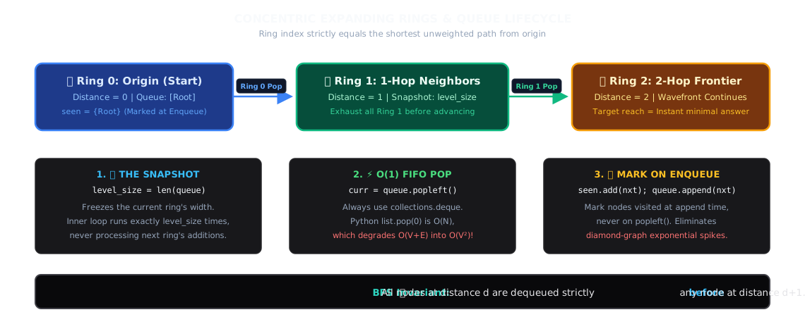
Drop a stone into still water: the ripple expands outward in uniform concentric rings. The wave reaches every point at distance 1 before it touches any point at distance 2, and every point at distance 2 before anything at distance 3. BFS is that exact physical wavefront.
At the core of BFS is a FIFO Queue (collections.deque), a synchronized clock (steps), and an enqueue-time deduplication guard (visited set).
The 3-Step BFS Operational Cycle
Every iteration of BFS executes three disciplined moves:
- 📸 The Freeze (Snapshot):
level_size = len(queue)locks the boundary of Ring . The inner loop iterates exactlylevel_sizetimes, completely clearing all distance- nodes before touching newly enqueued distance- nodes. - ⚡ The FIFO Drain:
curr = queue.popleft()pops nodes in strict first-in-first-out arrival order. - 🚫 Discover & Mark (Mark on Enqueue): For each valid, unvisited neighbor
nxt, you immediately executeseen.add(nxt)andqueue.append(nxt). Marking the neighbor at the moment of discovery—rather than when it is popped—permanently prevents duplicate queue insertions across diamond graphs.
The Shortest Path Guarantee
The Shortest Path Invariant: On an unweighted graph, all nodes at distance are dequeued and processed strictly before any node at distance . Therefore, the very first time the wavefront touches target node , the path length is mathematically guaranteed to be minimal.
The enqueue-time rule to say out loud: "I mark nodes as visited the moment they are appended to the queue, so each node enters the queue once. Marking on pop also works if I skip nodes that are already visited when I pop them, but then the queue can hold up to E entries; forgetting that skip is what makes the work blow up on diamond-shaped graphs."
🔬 Variable Anatomy: The 7 Variables Every BFS Uses
To connect abstract concepts with concrete Python syntax, here is the universal code anatomy showing what every variable does:
from collections import dequefrom typing import Any, Callable def bfsMasterTemplate( start_nodes: list[Any], get_neighbors: Callable[[Any], list[Any]], is_goal: Callable[[Any], bool], is_valid: Callable[[Any], bool]) -> int: # ========================================================================= # 1. THE STORAGE & QUEUING PIPELINE # ========================================================================= queue = deque(start_nodes) # 🧵 FIFO Pipeline: strictly processes d before d+1 visited = set(start_nodes) # 🚫 Visited Set: deduplication guard (MARK ON ENQUEUE!) steps = 0 # ⏱️ Clock / Distance: ring index equals shortest path # ========================================================================= # 2. THE WAVEFRONT PROCESSING LOOP # ========================================================================= while queue: level_size = len(queue) # 📸 THE SNAPSHOT: freezes breadth of current ring # --- A. DRAIN EXACTLY THIS RING --- for _ in range(level_size): curr = queue.popleft() # ⚡ O(1) front pop (NEVER use list.pop(0)!) # --- B. GOAL CHECK --- if is_goal(curr): return steps # 🎯 Shortest distance reached! # --- C. NEIGHBOR EXPANSION --- for nxt in get_neighbors(curr): # Guard: cycle prevention and boundary validation if nxt not in visited and is_valid(nxt): visited.add(nxt) # ⚠️ CRITICAL: Mark seen HERE on enqueue! queue.append(nxt) # Push to back of line (ring d+1) steps += 1 # 🌊 Advance concentric wavefront to next distance ring return -1 # ❌ Target unreachable Variable Role Reference:
| Variable | Role in Code | Question It Answers | ❌ What Happens If Omitted or Mismanaged? |
|---|---|---|---|
queue | collections.deque | "Which nodes are next in line at distance or ?" | ❌ Using list.pop(0) is , degrading traversal to an unacceptable . |
visited | Hash set or mutated grid | "Have I already scheduled this node in an earlier ring?" | ❌ Marking on popleft() instead of append() lets the same node be enqueued once per incoming edge (up to E entries); without a skip when it is popped, each copy is expanded again, so a node can be expanded many times instead of once. |
level_size | Snapshot integer | "How many nodes belong strictly to the current distance ring?" | ❌ Without snapshotting len(queue) before the inner loop, level boundaries collapse into a flat queue with lost step counts. |
directions | Coordinate delta vectors | "What are the legal steps from this grid coordinate?" | ❌ Forgetting diagonals in an 8-direction problem (LC 1091) or including them in a 4-direction problem (LC 994) yields incorrect paths. |
in_degree | Integer array / map | "How many prerequisite edges block this node from running?" | ❌ In Topological Sort (Kahn's), without in_degree, dependency chains cannot be resolved in valid topological order. |
q1, q2 | Dual frontier sets | "Which search frontier is currently smaller?" | ❌ In Bidirectional BFS, expanding the large frontier instead of the smaller one ruins the exponential optimization. |
0-1 Deque | Double-ended queue | "Does this edge transition cost 0 or 1?" | ❌ Using a Priority Queue () when edge weights are strictly 0 or 1 adds unnecessary logarithmic overhead over linear 0-1 BFS. |
🌟 The 3 Dimensions of BFS & The "Expanding Ripple" Principle
Just as Backtracking is governed by Depth, Choices, and Constraints, Breadth-First Search is defined by the 3 Dimensions of BFS:
- The Wavefront Ring = Distance / Depth
level_size = len(queue)snapshots the active ring before child additions grow the queue.- Question it answers: "How many steps / hops from the starting origin?"
- The Neighbor Generator = The Choices
get_neighbors(curr)expands the current frontier into adjacent unvisited nodes.- Question it answers: "Where can I legally step next from here?"
- The Visited Filter & In-Degree = The Constraints
nxt not in visitedorin_degree[nxt] == 0prevents cycles and blocks premature execution.- Question it answers: "Is this neighbor legal and unvisited?"
🎯 The 5 Essential BFS Paradigms & Archetypes
| Archetype | State Management | Enqueue / Wavefront Rule | Invariant / Pruning |
|---|---|---|---|
| 1. Level Snapshot (LC 102 / 103 / 199) | level_size = len(q) inner loop | Single-source root; enqueue children left/right | Group nodes strictly by depth; early exit on first leaf (111) |
| 2. 2D Grid Shortest (LC 1091 / Knight) | (r, c, dist) tuple or ring counter | 4-way or 8-way delta vectors | Mark visited in-place on grid; first arrival at (N-1, N-1) wins |
| 3. Multi-Source (LC 994 / LC 286) | Queue seeded with ALL sources at t=0 | Synchronized simultaneous infection wave | All origins start at t=0; decrement fresh count on enqueue |
| 4. Bidirectional BFS (LC 127 Word Ladder) | Two active frontiers q1 and q2 | Expand ALWAYS the smaller frontier (len(q1) > len(q2)) | Exponential collapse: |
| 5. Topological Sort (LC 207 / 210 Kahn) | in_degree array + adjacency list | Seed queue with in-degree 0 | Decrement in-degree of neighbors; if popped < V Cycle! |
Understanding Invariants: Concentric Wavefront & Enqueue Deduplication
At any instant, the FIFO queue contains nodes exclusively of distance d and d + 1. The first time a node is touched and enqueued, its shortest path from the source is permanently guaranteed.
Breadth-First Search processes graph vertices in monotonic ring-by-ring order. By freezing the level size at the start of each ring and marking neighbors as visited at the moment of enqueue, BFS guarantees minimal path discovery in O(V + E) time with each node enqueued once.
Marking on enqueue rather than dequeue guarantees each vertex enters the queue at most once, so the queue never holds duplicate copies of a node.
Because rings expand in monotonically non-decreasing distance order, the first encounter with target T is mathematically guaranteed to be the shortest path.
Common Questions
"Why do we need level_size = len(queue) before the inner loop — isn't just draining the queue with a while queue: loop enough to visit everything in BFS order?"
A plain
while queue:loop does visit every node in the correct overall order — but it destroys the one thing level-order problems actually need: knowing where one ring ends and the next begins.Without the snapshot, nodes from distance and distance sit in the same undifferentiated queue. A child gets enqueued (at distance ) while its own siblings (still distance ) are still waiting in line ahead of it — so by the time you've drained the whole queue, you have one flat list of every node ever visited, with no marker for which ones belonged together.
level_size = len(queue)freezes that boundary before any enqueuing happens this round: "exactly this many nodes belong to ring ." The innerfor _ in range(level_size):loop then drains precisely those nodes and no others — any children it enqueues land safely at the back, behind the rest of the current ring, and only get touched on the next outer iteration. That single line is what turns a flat FIFO drain into discrete, groupable levels — it costs nothing extra algorithmically (stillO(N)total), it just captures information a plainwhile queue:throws away.
Coach discussion points
- 1.
"You mark a node visited when you pop it off the queue. Draw a small diamond graph () and explain why is enqueued twice."
- 2.
"Why does the first time BFS reaches a node guarantee the shortest path? What mathematical property breaks if edges have varying positive weights?"
- 3.
"In Open the Lock, why does treating each 4-digit combination as a node in an implicit 10,000-node graph make this a BFS problem rather than a simulation problem?"
- 4.
"In Word Ladder, why does expanding the smaller frontier in Bidirectional BFS reduce complexity from to ?"
- 5.
"In Knight Shortest Path, the coordinate space is technically unbounded — why doesn't that break BFS's shortest-path guarantee, and what data structure choice makes an unbounded visited-set practical?"
- 6.
"In Sliding Puzzle, why does serializing the board into a string matter more here than in a grid problem like Rotting Oranges, where you can just mutate the grid in place?"
- 7.
"In Word Ladder II, why is removing a discovered word from the candidate pool immediately (per-word) wrong, while removing it once per layer (batched) is correct? Walk through a case with two parents in the same layer reaching the same child word."
- 8.
"Word Ladder II runs two separate traversals — a BFS and then a backtracking DFS. Why can't the BFS alone produce the final list of paths, and what does the
parentsmap actually represent structurally?"
Complexity analysis
Theoretical Big-O Derivations
Time Complexity:
- Every vertex enters the queue at most once and is popped in time with
deque.popleft(). - For each popped vertex, every outgoing edge is examined once (or twice in undirected graphs).
- Grid Specialization (): , and each cell has at most 4 (or 8) edges. Total time: .
- Word Ladder Specialization: , and checking 26 letter replacements takes per word. Total time: .
- Word Ladder II Specialization: Same BFS layering cost as Word Ladder, plus an additional backtracking DFS pass to emit all shortest paths of length up to each: total .
- Sliding Puzzle Specialization: The board has a fixed, tiny cell count (here ), so the state space is bounded by permutations regardless of input; each state generates at most 4 neighbor swaps in time each: total .
Space Complexity: where is Maximum Width
- The memory consumed is bounded by the widest ring in the graph.
- For a balanced binary tree, the leaf level holds nodes memory.
- For a skewed linear tree, each ring holds 1 node memory.
DFS vs. BFS Architectural Trade-Off Table
| Metric / Dimension | Depth-First Search (DFS) | Breadth-First Search (BFS) |
|---|---|---|
| Auxiliary Data Structure | Implicit Call Stack (Recursion) or explicit LIFO Stack | Explicit FIFO Queue (collections.deque) |
| Space Complexity | where is Tree Height | where is Max Level Width |
| Worst-Case Space Input | Skewed / Degenerate linked list () | Balanced Tree with massive leaf breadth () |
| Shortest Path Guarantee? | ❌ No (Explores deeply along arbitrary branches) | ✅ Yes (On unweighted graphs, first arrival is optimal) |
| Ideal Problem Domain | Exhaustive search, permutations, subtree aggregation, backtracks | Shortest path, fewest turns, level-order grouping, wavefronts |
Real-World Distributed Systems Applications
- Distributed Web Crawlers & Search Indexing (Googlebot / Apache Nutch):
- Web crawlers execute bounded-depth multi-source BFS to discover, fetch, and index web pages across hyperlinked domains while adhering to per-host crawl delay policies.
- Social Graph Proximity & Degrees of Separation (LinkedIn / Facebook):
- Graph databases execute bidirectional BFS to calculate 1st, 2nd, and 3rd-degree connection recommendations between users in sub-second latency.
- Network Switch Spanning Tree Protocol (STP / IEEE 802.1D):
- Ethernet bridge switches broadcast BPDU packets via BFS wavefronts to compute loop-free spanning trees across physical network topologies.
- Game AI Pathfinding & Navigation Meshes (NavMesh Wavefront):
- Game engines run multi-source BFS over 2D/3D navigation grid meshes to calculate tactical squad movement paths toward target objectives.
A routing table computing hop count, a chess engine solving "mate in N", and a package manager measuring how many dependency levels deep a transitive dependency sits all lean on the same ring-expansion idea: explore everything one step away, then everything two steps away, stopping the instant the target turns up. The ring number is the answer — the same idea a social network uses to answer "how many degrees of separation" without checking billions of friendship chains.
💡 Don't worry if queue state tracking feels unfamiliar right now! BFS is one core concentric wavefront mechanism: freezing level_size = len(queue) and marking nodes in visited immediately upon enqueue. As you progress through the Archetype Variants (from Level-Order Traversal and Rotting Oranges to Word Ladder and Multi-Source Grids), each hands-on challenge will cement this intuition until writing clean queue loops and shortest-path guarantees becomes second nature.
The Python list trap: Calling
queue.pop(0)on a standard Python list shifts all remaining elements on every pop, turning an traversal into . Always usecollections.deque.popleft().Missing
level_sizesnapshot: Mutating the queue inside the level loop without taking a snapshot oflen(queue)collapses multiple tree depth levels into a single flat array.Enqueuing null pointers: Pushing
node.leftornode.rightwithout checkingif node.left:fills the queue withNoneelements that crash child property access on the next level.
Staff+ Systems Architecture & Hardware Considerations
Triggers: "shortest path in unweighted graph", "minimum moves / operations", "level-by-level traversal", "nearest 0/1 multi-source flood fill". Breadth-first exploration radiating concentrically outward from sources.
Graph with vertices and edges. Time budget is as every vertex and edge is enqueued and dequeued at most once. Auxiliary space is bounded by the maximum frontier breadth , up to .
Marking nodes as visited when dequeuing rather than enqueuing (causes identical nodes to be added to the queue exponentially, blowing up memory to ); using a flat array list.pop(0) ( shift) instead of a circular buffer or double-ended queue collections.deque ( popleft).
Conceptual Foundation & Intuitive Analogy
🧭 Conceptual Foundation & Pattern Intuition
Breadth-First Search (BFS) explores tree or graph topologies by expanding outward in concentric generational waves. While Depth-First Search charges blindly down a single path until hitting a dead end, BFS visits every vertex at distance before touching any vertex at distance . In a binary tree, BFS organizes nodes into discrete horizontal levels. The fundamental architectural mechanism that makes level-order grouping possible is the queue snapshot: taking level_size = len(queue) before the inner loop starts, ensuring that newly enqueued child nodes belonging to the next generation are never processed during the current level's sweep.
🏟️ The Analogy: Dropping a Pebble into a Calm Pond
Imagine dropping a small pebble into the center of a glass-smooth pond. The impact creates ripples that expand outward in concentric circles. The first ripple hits all nearby water bugs simultaneously. A second later, the second ring expands further out, hitting the next ring of bugs. BFS behaves exactly like this water ripple: the root is the pebble drop, and each iteration of the outer loop processes exactly one concentric ring of children across the entire breadth of the tree.
🔑 Why It Works
Because a binary tree is an acyclic hierarchy, no node can ever be reached by two different paths. Consequently, tree BFS requires no visited set, executing in pure time and consuming space, where is the maximum tree width (at most at the lowest level).
The invariant to say out loud: "At any instant, my queue holds nodes exclusively of distance d and d+1, never more. The first time a node is touched, I have strictly found its shortest path."
Nodes enter queue in monotonically non-decreasing order of path distance. Evaluates level_size = len(queue) to process discrete tiers.
while queue: for _ in range(len(queue)): popleft(), enqueue unvisited neighbors.
The Mental Model of Breadth-First Search
Identify the state expansion wavefront and queue structure before coding.
1Level-Order BFS
root ➔ freeze level_size = len(queue) ➔ batch process ringLevel Order Traversal (BFS by Level)
| 1 | from collections import deque |
| 2 | from typing import Callable, Iterable, List, Optional, TypeVar |
| 3 | |
| 4 | Item = TypeVar("Item") |
| 5 | |
| 6 | class TreeNode: |
| 7 | def __init__(self, val: int = 0, left: Optional["TreeNode"] = None, right: Optional["TreeNode"] = None): |
| 8 | self.val = val |
| 9 | self.left = left |
| 10 | self.right = right |
| 11 | |
| 12 | |
| 13 | def level_by_level(start: Iterable[Item], children: Callable[[Item], Iterable[Item]], record: Callable[[List[Item]], None]) -> None: |
| 14 | """Level-Order BFS: hand the nodes of each level, left to right, to record(level), level after level. |
| 15 | start is the first level. children(node) lists the nodes of the next level below node. |
| 16 | Precondition: every node is reached once, as in a tree, or children skips the nodes already seen. |
| 17 | V = the nodes. W = the largest level. T = the cost of one children call, or of record for one node. |
| 18 | Time: O(V * T) | Space: O(W) queue and current level |
| 19 | """ |
| 20 | queue = deque(start) # holds nodes queued for this or a later level, in enqueue order |
| 21 | |
| 22 | while queue: |
| 23 | # 1. Snapshot the Level Boundary: |
| 24 | # len(queue) right now counts only nodes queued from the previous level, so |
| 25 | # freezing it before the inner loop keeps this level's own children out of |
| 26 | # the current sweep. |
| 27 | level_size = len(queue) |
| 28 | current_level = [] |
| 29 | |
| 30 | for _ in range(level_size): |
| 31 | # 2. Pop and Record This Level's Node: |
| 32 | # popleft() returns nodes in the order they were queued, so the |
| 33 | # earliest-queued node is always processed first. |
| 34 | node = queue.popleft() |
| 35 | current_level.append(node) |
| 36 | queue.extend(children(node)) |
| 37 | |
| 38 | # 3. Record the Completed Level: |
| 39 | record(current_level) |
Read len(queue) into level_size at the start of each round: exactly that many nodes belong to the current level. Process only those, adding their children, and the queue then holds just the next level. That gives level boundaries without storing a depth per node. The trap is re-reading the size while children arrive: the queue grows during the round, so a bound that checks len(queue) again (a while loop, or a loop in another language) runs on into the next level; freeze it in level_size first.
Gotcha 1 of 4
- The trap
Gotcha 1: Looping
while queueinside the roundMistakewhile queue:Fixfor _ in range(level_size):What happens: Children are added to the back of
queueduring the round.while queuekeeps popping them in the same round. So the loop runs on into the next level, and every node ends up in one list.level_size = len(queue)is read once, before any child is added. The inner loop runs exactly that many times.Example: Binary Tree Level Order Traversal (LC 102): root = [3,9,20,null,null,15,7]Mistake: returns [[3, 9, 20, 15, 7]]Fix: returns [[3], [9, 20], [15, 7]]
Built on the mental models above
- Topological SortTopological Sort (Kahn's Algorithm)
An in-degree count per node decides when a node may enter
queue. - Multi-Source BFSMulti-Source BFS
Every source starts in
queueat the same time, so all sources spread together. - Graph BFSBFS on a Graph (Mark on Push)
A
seenset marks a node when it is added toqueue, so a node with two parents is expanded once and a cycle ends. - Shortest-Path BFSShortest Path BFS (Unweighted Grid / Graph)
Each node also stores
dist, the number of moves from the start, which is the fewest because BFS reaches nodes in order of distance. - Zero-One BFS0-1 BFS
A deque holds the queue: a move that costs 0 goes to the front and a move that costs 1 goes to the back.
- State-Space BFSBFS on an Implicit State Graph (incl. Bidirectional BFS)
A node is a whole configuration, and its neighbours are built by changing it a little.
The BFS Decision Rule
When facing an unseen graph, grid, or state-space problem, ask in this order:
Freeze level_size = len(queue) and process exactly that many nodes per level.
Mark a node in seen at the moment you add it to queue, so each node is queued once.
Enqueue all sources at distance 0 before starting the loop.
Mark a cell visited when you enqueue it; the first time the target is reached, its distance is the answer.
Build each configuration's neighbours yourself, keep a visited set of configurations, and search from both ends when the branching is large.
Use deque: appendleft for 0-weight edges, append for 1-weight edges.
Queue every node with in-degree 0 and lower each neighbour's in-degree as you pop; fewer than n popped means a cycle.
Pattern Architecture & Invariant Design Masterclass
Drop a stone into still water: the ripple expands outward in uniform concentric rings. The wave reaches every point at distance 1 before it touches any point at distance 2, and every point at distance 2 before anything at distance 3. BFS is that exact physical wavefront.
At the core of BFS is a FIFO Queue (collections.deque), a synchronized clock (steps), and an enqueue-time deduplication guard (visited set).
The 3-Step BFS Operational Cycle
Every iteration of BFS executes three disciplined moves:
- 📸 The Freeze (Snapshot):
level_size = len(queue)locks the boundary of Ring . The inner loop iterates exactlylevel_sizetimes, completely clearing all distance- nodes before touching newly enqueued distance- nodes. - ⚡ The FIFO Drain:
curr = queue.popleft()pops nodes in strict first-in-first-out arrival order. - 🚫 Discover & Mark (Mark on Enqueue): For each valid, unvisited neighbor
nxt, you immediately executeseen.add(nxt)andqueue.append(nxt). Marking the neighbor at the moment of discovery—rather than when it is popped—permanently prevents duplicate queue insertions across diamond graphs.
The Shortest Path Guarantee
The Shortest Path Invariant: On an unweighted graph, all nodes at distance are dequeued and processed strictly before any node at distance . Therefore, the very first time the wavefront touches target node , the path length is mathematically guaranteed to be minimal.
The enqueue-time rule to say out loud: "I mark nodes as visited the moment they are appended to the queue, so each node enters the queue once. Marking on pop also works if I skip nodes that are already visited when I pop them, but then the queue can hold up to E entries; forgetting that skip is what makes the work blow up on diamond-shaped graphs."
🔬 Variable Anatomy: The 7 Variables Every BFS Uses
To connect abstract concepts with concrete Python syntax, here is the universal code anatomy showing what every variable does:
from collections import dequefrom typing import Any, Callable def bfsMasterTemplate( start_nodes: list[Any], get_neighbors: Callable[[Any], list[Any]], is_goal: Callable[[Any], bool], is_valid: Callable[[Any], bool]) -> int: # ========================================================================= # 1. THE STORAGE & QUEUING PIPELINE # ========================================================================= queue = deque(start_nodes) # 🧵 FIFO Pipeline: strictly processes d before d+1 visited = set(start_nodes) # 🚫 Visited Set: deduplication guard (MARK ON ENQUEUE!) steps = 0 # ⏱️ Clock / Distance: ring index equals shortest path # ========================================================================= # 2. THE WAVEFRONT PROCESSING LOOP # ========================================================================= while queue: level_size = len(queue) # 📸 THE SNAPSHOT: freezes breadth of current ring # --- A. DRAIN EXACTLY THIS RING --- for _ in range(level_size): curr = queue.popleft() # ⚡ O(1) front pop (NEVER use list.pop(0)!) # --- B. GOAL CHECK --- if is_goal(curr): return steps # 🎯 Shortest distance reached! # --- C. NEIGHBOR EXPANSION --- for nxt in get_neighbors(curr): # Guard: cycle prevention and boundary validation if nxt not in visited and is_valid(nxt): visited.add(nxt) # ⚠️ CRITICAL: Mark seen HERE on enqueue! queue.append(nxt) # Push to back of line (ring d+1) steps += 1 # 🌊 Advance concentric wavefront to next distance ring return -1 # ❌ Target unreachable Variable Role Reference:
| Variable | Role in Code | Question It Answers | ❌ What Happens If Omitted or Mismanaged? |
|---|---|---|---|
queue | collections.deque | "Which nodes are next in line at distance or ?" | ❌ Using list.pop(0) is , degrading traversal to an unacceptable . |
visited | Hash set or mutated grid | "Have I already scheduled this node in an earlier ring?" | ❌ Marking on popleft() instead of append() lets the same node be enqueued once per incoming edge (up to E entries); without a skip when it is popped, each copy is expanded again, so a node can be expanded many times instead of once. |
level_size | Snapshot integer | "How many nodes belong strictly to the current distance ring?" | ❌ Without snapshotting len(queue) before the inner loop, level boundaries collapse into a flat queue with lost step counts. |
directions | Coordinate delta vectors | "What are the legal steps from this grid coordinate?" | ❌ Forgetting diagonals in an 8-direction problem (LC 1091) or including them in a 4-direction problem (LC 994) yields incorrect paths. |
in_degree | Integer array / map | "How many prerequisite edges block this node from running?" | ❌ In Topological Sort (Kahn's), without in_degree, dependency chains cannot be resolved in valid topological order. |
q1, q2 | Dual frontier sets | "Which search frontier is currently smaller?" | ❌ In Bidirectional BFS, expanding the large frontier instead of the smaller one ruins the exponential optimization. |
0-1 Deque | Double-ended queue | "Does this edge transition cost 0 or 1?" | ❌ Using a Priority Queue () when edge weights are strictly 0 or 1 adds unnecessary logarithmic overhead over linear 0-1 BFS. |
🌟 The 3 Dimensions of BFS & The "Expanding Ripple" Principle
Just as Backtracking is governed by Depth, Choices, and Constraints, Breadth-First Search is defined by the 3 Dimensions of BFS:
- The Wavefront Ring = Distance / Depth
level_size = len(queue)snapshots the active ring before child additions grow the queue.- Question it answers: "How many steps / hops from the starting origin?"
- The Neighbor Generator = The Choices
get_neighbors(curr)expands the current frontier into adjacent unvisited nodes.- Question it answers: "Where can I legally step next from here?"
- The Visited Filter & In-Degree = The Constraints
nxt not in visitedorin_degree[nxt] == 0prevents cycles and blocks premature execution.- Question it answers: "Is this neighbor legal and unvisited?"
🎯 The 5 Essential BFS Paradigms & Archetypes
| Archetype | State Management | Enqueue / Wavefront Rule | Invariant / Pruning |
|---|---|---|---|
| 1. Level Snapshot (LC 102 / 103 / 199) | level_size = len(q) inner loop | Single-source root; enqueue children left/right | Group nodes strictly by depth; early exit on first leaf (111) |
| 2. 2D Grid Shortest (LC 1091 / Knight) | (r, c, dist) tuple or ring counter | 4-way or 8-way delta vectors | Mark visited in-place on grid; first arrival at (N-1, N-1) wins |
| 3. Multi-Source (LC 994 / LC 286) | Queue seeded with ALL sources at t=0 | Synchronized simultaneous infection wave | All origins start at t=0; decrement fresh count on enqueue |
| 4. Bidirectional BFS (LC 127 Word Ladder) | Two active frontiers q1 and q2 | Expand ALWAYS the smaller frontier (len(q1) > len(q2)) | Exponential collapse: |
| 5. Topological Sort (LC 207 / 210 Kahn) | in_degree array + adjacency list | Seed queue with in-degree 0 | Decrement in-degree of neighbors; if popped < V Cycle! |
Understanding Invariants: Concentric Wavefront & Enqueue Deduplication
At any instant, the FIFO queue contains nodes exclusively of distance d and d + 1. The first time a node is touched and enqueued, its shortest path from the source is permanently guaranteed.
Breadth-First Search processes graph vertices in monotonic ring-by-ring order. By freezing the level size at the start of each ring and marking neighbors as visited at the moment of enqueue, BFS guarantees minimal path discovery in O(V + E) time with each node enqueued once.
Marking on enqueue rather than dequeue guarantees each vertex enters the queue at most once, so the queue never holds duplicate copies of a node.
Because rings expand in monotonically non-decreasing distance order, the first encounter with target T is mathematically guaranteed to be the shortest path.
Common Questions
"Why do we need level_size = len(queue) before the inner loop — isn't just draining the queue with a while queue: loop enough to visit everything in BFS order?"
A plain
while queue:loop does visit every node in the correct overall order — but it destroys the one thing level-order problems actually need: knowing where one ring ends and the next begins.Without the snapshot, nodes from distance and distance sit in the same undifferentiated queue. A child gets enqueued (at distance ) while its own siblings (still distance ) are still waiting in line ahead of it — so by the time you've drained the whole queue, you have one flat list of every node ever visited, with no marker for which ones belonged together.
level_size = len(queue)freezes that boundary before any enqueuing happens this round: "exactly this many nodes belong to ring ." The innerfor _ in range(level_size):loop then drains precisely those nodes and no others — any children it enqueues land safely at the back, behind the rest of the current ring, and only get touched on the next outer iteration. That single line is what turns a flat FIFO drain into discrete, groupable levels — it costs nothing extra algorithmically (stillO(N)total), it just captures information a plainwhile queue:throws away.
Coach discussion points
- 1.
"You mark a node visited when you pop it off the queue. Draw a small diamond graph () and explain why is enqueued twice."
- 2.
"Why does the first time BFS reaches a node guarantee the shortest path? What mathematical property breaks if edges have varying positive weights?"
- 3.
"In Open the Lock, why does treating each 4-digit combination as a node in an implicit 10,000-node graph make this a BFS problem rather than a simulation problem?"
- 4.
"In Word Ladder, why does expanding the smaller frontier in Bidirectional BFS reduce complexity from to ?"
- 5.
"In Knight Shortest Path, the coordinate space is technically unbounded — why doesn't that break BFS's shortest-path guarantee, and what data structure choice makes an unbounded visited-set practical?"
- 6.
"In Sliding Puzzle, why does serializing the board into a string matter more here than in a grid problem like Rotting Oranges, where you can just mutate the grid in place?"
- 7.
"In Word Ladder II, why is removing a discovered word from the candidate pool immediately (per-word) wrong, while removing it once per layer (batched) is correct? Walk through a case with two parents in the same layer reaching the same child word."
- 8.
"Word Ladder II runs two separate traversals — a BFS and then a backtracking DFS. Why can't the BFS alone produce the final list of paths, and what does the
parentsmap actually represent structurally?"
Complexity analysis
Theoretical Big-O Derivations
Time Complexity:
- Every vertex enters the queue at most once and is popped in time with
deque.popleft(). - For each popped vertex, every outgoing edge is examined once (or twice in undirected graphs).
- Grid Specialization (): , and each cell has at most 4 (or 8) edges. Total time: .
- Word Ladder Specialization: , and checking 26 letter replacements takes per word. Total time: .
- Word Ladder II Specialization: Same BFS layering cost as Word Ladder, plus an additional backtracking DFS pass to emit all shortest paths of length up to each: total .
- Sliding Puzzle Specialization: The board has a fixed, tiny cell count (here ), so the state space is bounded by permutations regardless of input; each state generates at most 4 neighbor swaps in time each: total .
Space Complexity: where is Maximum Width
- The memory consumed is bounded by the widest ring in the graph.
- For a balanced binary tree, the leaf level holds nodes memory.
- For a skewed linear tree, each ring holds 1 node memory.
DFS vs. BFS Architectural Trade-Off Table
| Metric / Dimension | Depth-First Search (DFS) | Breadth-First Search (BFS) |
|---|---|---|
| Auxiliary Data Structure | Implicit Call Stack (Recursion) or explicit LIFO Stack | Explicit FIFO Queue (collections.deque) |
| Space Complexity | where is Tree Height | where is Max Level Width |
| Worst-Case Space Input | Skewed / Degenerate linked list () | Balanced Tree with massive leaf breadth () |
| Shortest Path Guarantee? | ❌ No (Explores deeply along arbitrary branches) | ✅ Yes (On unweighted graphs, first arrival is optimal) |
| Ideal Problem Domain | Exhaustive search, permutations, subtree aggregation, backtracks | Shortest path, fewest turns, level-order grouping, wavefronts |
Real-World Distributed Systems Applications
- Distributed Web Crawlers & Search Indexing (Googlebot / Apache Nutch):
- Web crawlers execute bounded-depth multi-source BFS to discover, fetch, and index web pages across hyperlinked domains while adhering to per-host crawl delay policies.
- Social Graph Proximity & Degrees of Separation (LinkedIn / Facebook):
- Graph databases execute bidirectional BFS to calculate 1st, 2nd, and 3rd-degree connection recommendations between users in sub-second latency.
- Network Switch Spanning Tree Protocol (STP / IEEE 802.1D):
- Ethernet bridge switches broadcast BPDU packets via BFS wavefronts to compute loop-free spanning trees across physical network topologies.
- Game AI Pathfinding & Navigation Meshes (NavMesh Wavefront):
- Game engines run multi-source BFS over 2D/3D navigation grid meshes to calculate tactical squad movement paths toward target objectives.
A routing table computing hop count, a chess engine solving "mate in N", and a package manager measuring how many dependency levels deep a transitive dependency sits all lean on the same ring-expansion idea: explore everything one step away, then everything two steps away, stopping the instant the target turns up. The ring number is the answer — the same idea a social network uses to answer "how many degrees of separation" without checking billions of friendship chains.
💡 Don't worry if queue state tracking feels unfamiliar right now! BFS is one core concentric wavefront mechanism: freezing level_size = len(queue) and marking nodes in visited immediately upon enqueue. As you progress through the Archetype Variants (from Level-Order Traversal and Rotting Oranges to Word Ladder and Multi-Source Grids), each hands-on challenge will cement this intuition until writing clean queue loops and shortest-path guarantees becomes second nature.
The Python list trap: Calling
queue.pop(0)on a standard Python list shifts all remaining elements on every pop, turning an traversal into . Always usecollections.deque.popleft().Missing
level_sizesnapshot: Mutating the queue inside the level loop without taking a snapshot oflen(queue)collapses multiple tree depth levels into a single flat array.Enqueuing null pointers: Pushing
node.leftornode.rightwithout checkingif node.left:fills the queue withNoneelements that crash child property access on the next level.
Staff+ Systems Architecture & Hardware Considerations
Triggers: "shortest path in unweighted graph", "minimum moves / operations", "level-by-level traversal", "nearest 0/1 multi-source flood fill". Breadth-first exploration radiating concentrically outward from sources.
Graph with vertices and edges. Time budget is as every vertex and edge is enqueued and dequeued at most once. Auxiliary space is bounded by the maximum frontier breadth , up to .
Marking nodes as visited when dequeuing rather than enqueuing (causes identical nodes to be added to the queue exponentially, blowing up memory to ); using a flat array list.pop(0) ( shift) instead of a circular buffer or double-ended queue collections.deque ( popleft).